7  Time Series Spillover - GVAR

7.1 Library

library(Spillover)

Loading required package: vars

Loading required package: MASS

Loading required package: strucchange

Loading required package: zoo

Attaching package: 'zoo'

The following objects are masked from 'package:base':

    as.Date, as.Date.numeric

Loading required package: sandwich

Loading required package: urca

Loading required package: lmtest

library(vars)
library(urca)
library(splitstackshape)
library(igraph)

Attaching package: 'igraph'

The following objects are masked from 'package:stats':

    decompose, spectrum

The following object is masked from 'package:base':

    union

library(reshape)

7.2 Data: Diebold-Yilmaz 2012

data(dy2012)
head(dy2012)  # in log volatility form

        Date     Stocks      Bonds Commodities         FX
1 1999-01-25  -9.891998 -10.081905   -9.797694 -12.971578
2 1999-01-26  -9.353294 -10.090498  -11.475212 -13.237477
3 1999-01-27  -9.314619 -10.103319  -15.317140  -9.749465
4 1999-01-28  -8.997370 -10.090498  -12.044040 -10.853610
5 1999-01-29  -8.855955  -9.426092  -12.928477 -11.788281
6 1999-02-01 -10.282395  -8.936206  -12.821930 -11.308455

log volatility return: \[ \sigma^2_{it} = 0.361[ln(P^{max}_{i,t}) - ln(P^{min}_{i,t-1}))]^2 \]

\[ \sigma_{it} = 100*(\sqrt{252*\sigma^2_{it}}) \]

class(dy2012)

[1] "data.frame"

nrow(dy2012)

[1] 2771

7.3 VAR Model

PP.test(dy2012$Stocks)

    Phillips-Perron Unit Root Test

data:  dy2012$Stocks
Dickey-Fuller = -32.546, Truncation lag parameter = 9, p-value = 0.01

PP.test(dy2012$Bonds)

    Phillips-Perron Unit Root Test

data:  dy2012$Bonds
Dickey-Fuller = -41.249, Truncation lag parameter = 9, p-value = 0.01

PP.test(dy2012$Commodities)

    Phillips-Perron Unit Root Test

data:  dy2012$Commodities
Dickey-Fuller = -48.523, Truncation lag parameter = 9, p-value = 0.01

PP.test(dy2012$FX)

    Phillips-Perron Unit Root Test

data:  dy2012$FX
Dickey-Fuller = -47.527, Truncation lag parameter = 9, p-value = 0.01

# Optimum Lag
VARselect(dy2012[,-1], lag.max = 4, type = c("both"))

$selection
AIC(n)  HQ(n)  SC(n) FPE(n) 
     4      4      4      4 

$criteria
                 1          2          3          4
AIC(n) -0.11329876 -0.4490460 -0.5882320 -0.6679637
HQ(n)  -0.09473562 -0.4181074 -0.5449180 -0.6122743
SC(n)  -0.06190286 -0.3633861 -0.4683083 -0.5137760
FPE(n)  0.89288389  0.6382368  0.5553084  0.5127520

# VAR Model
VAR_4 <- VAR(dy2012[,-1], p=4)
VAR_4

VAR Estimation Results:
======================= 

Estimated coefficients for equation Stocks: 
=========================================== 
Call:
Stocks = Stocks.l1 + Bonds.l1 + Commodities.l1 + FX.l1 + Stocks.l2 + Bonds.l2 + Commodities.l2 + FX.l2 + Stocks.l3 + Bonds.l3 + Commodities.l3 + FX.l3 + Stocks.l4 + Bonds.l4 + Commodities.l4 + FX.l4 + const 

     Stocks.l1       Bonds.l1 Commodities.l1          FX.l1      Stocks.l2 
  0.1835084630  -0.0242487169  -0.0036337209   0.0219988664   0.2741423171 
      Bonds.l2 Commodities.l2          FX.l2      Stocks.l3       Bonds.l3 
  0.0027926328  -0.0108044031   0.0040316592   0.2025153665   0.0360740337 
Commodities.l3          FX.l3      Stocks.l4       Bonds.l4 Commodities.l4 
 -0.0158017651   0.0007938866   0.1620506569   0.0333733392  -0.0029608791 
         FX.l4          const 
 -0.0007384703  -1.3401330918 


Estimated coefficients for equation Bonds: 
========================================== 
Call:
Bonds = Stocks.l1 + Bonds.l1 + Commodities.l1 + FX.l1 + Stocks.l2 + Bonds.l2 + Commodities.l2 + FX.l2 + Stocks.l3 + Bonds.l3 + Commodities.l3 + FX.l3 + Stocks.l4 + Bonds.l4 + Commodities.l4 + FX.l4 + const 

     Stocks.l1       Bonds.l1 Commodities.l1          FX.l1      Stocks.l2 
   0.068141170    0.163772247    0.052592815    0.004319034    0.025511120 
      Bonds.l2 Commodities.l2          FX.l2      Stocks.l3       Bonds.l3 
   0.174716290    0.024936542    0.013962476    0.041353468    0.129894730 
Commodities.l3          FX.l3      Stocks.l4       Bonds.l4 Commodities.l4 
  -0.043136698    0.011844827   -0.026075514    0.218597337    0.039128430 
         FX.l4          const 
  -0.027491905   -1.080792116 


Estimated coefficients for equation Commodities: 
================================================ 
Call:
Commodities = Stocks.l1 + Bonds.l1 + Commodities.l1 + FX.l1 + Stocks.l2 + Bonds.l2 + Commodities.l2 + FX.l2 + Stocks.l3 + Bonds.l3 + Commodities.l3 + FX.l3 + Stocks.l4 + Bonds.l4 + Commodities.l4 + FX.l4 + const 

     Stocks.l1       Bonds.l1 Commodities.l1          FX.l1      Stocks.l2 
  -0.022755735    0.098201350    0.183333080    0.048298645   -0.013291588 
      Bonds.l2 Commodities.l2          FX.l2      Stocks.l3       Bonds.l3 
  -0.013132921    0.207410140    0.044188995   -0.049827512    0.004592325 
Commodities.l3          FX.l3      Stocks.l4       Bonds.l4 Commodities.l4 
   0.185198136   -0.037523992   -0.030251601    0.060251069    0.156050483 
         FX.l4          const 
   0.038706445   -1.543777242 


Estimated coefficients for equation FX: 
======================================= 
Call:
FX = Stocks.l1 + Bonds.l1 + Commodities.l1 + FX.l1 + Stocks.l2 + Bonds.l2 + Commodities.l2 + FX.l2 + Stocks.l3 + Bonds.l3 + Commodities.l3 + FX.l3 + Stocks.l4 + Bonds.l4 + Commodities.l4 + FX.l4 + const 

     Stocks.l1       Bonds.l1 Commodities.l1          FX.l1      Stocks.l2 
    0.06467245    -0.01930672     0.02517504     0.06996402     0.03590206 
      Bonds.l2 Commodities.l2          FX.l2      Stocks.l3       Bonds.l3 
   -0.02073267     0.01066279     0.20847309    -0.01249224     0.03780188 
Commodities.l3          FX.l3      Stocks.l4       Bonds.l4 Commodities.l4 
   -0.00393800     0.18185464    -0.01552454     0.05072537     0.01667104 
         FX.l4          const 
    0.11443511    -2.99838336 

7.4 Volatility Spillover DY-2012

# Total Spillover Index
sp <- G.spillover(VAR_4, n.ahead = 10, standardized = F )
sp

                               Stocks     Bonds Commodities        FX
Stocks                      88.757002  7.291185   0.3453279  3.606486
Bonds                       10.213545 81.445712   2.7269737  5.613770
Commodities                  0.468118  3.695953  93.6941893  2.141740
FX                           5.691579  7.026017   1.5477592 85.734645
C. to others (spillover)    16.373241 18.013154   4.6200608 11.361996
C. to others including own 105.130243 99.458866  98.3142500 97.096641
                           C. from others
Stocks                          11.242998
Bonds                           18.554288
Commodities                      6.305811
FX                              14.265355
C. to others (spillover)        12.592113
C. to others including own     400.000000

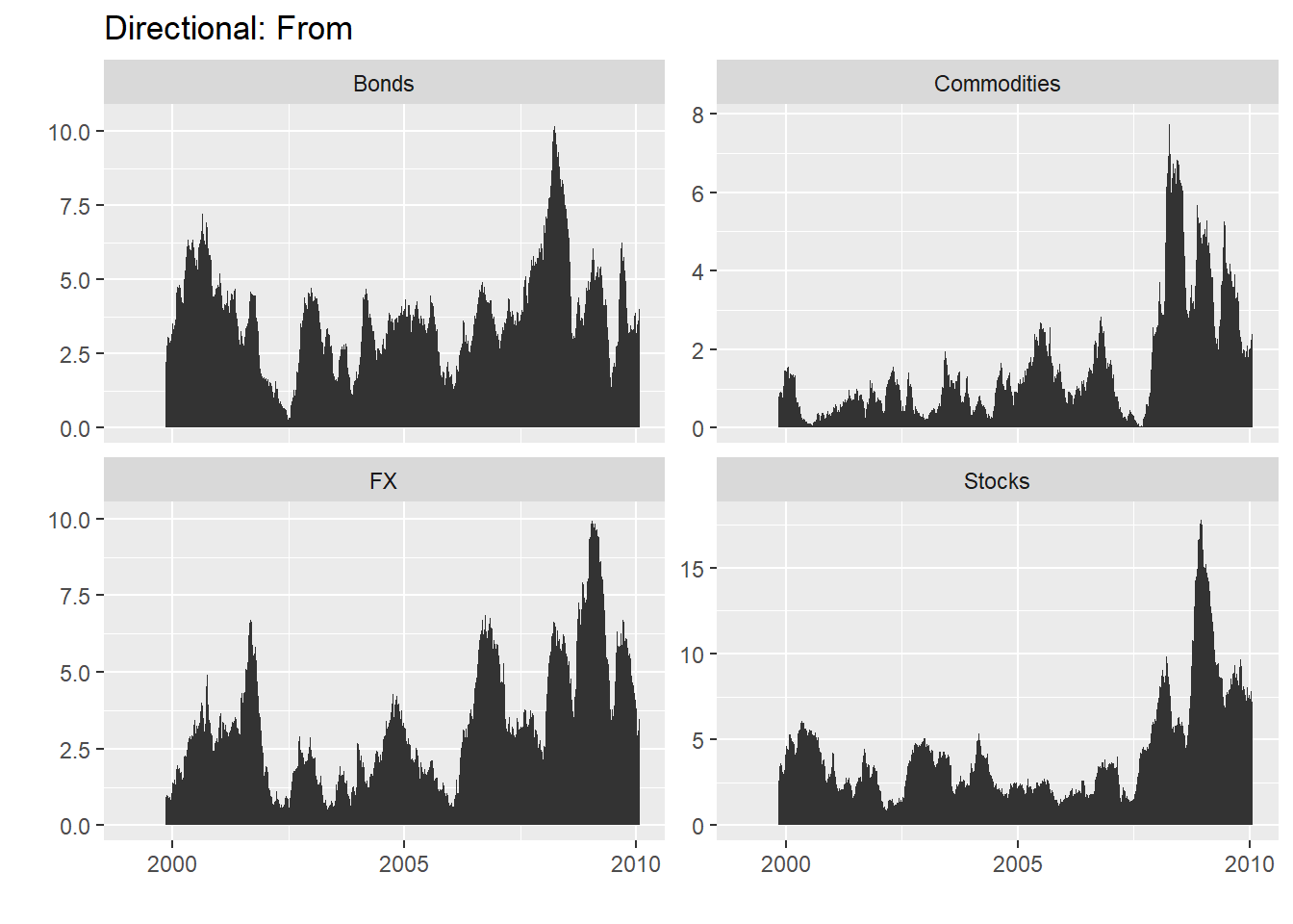
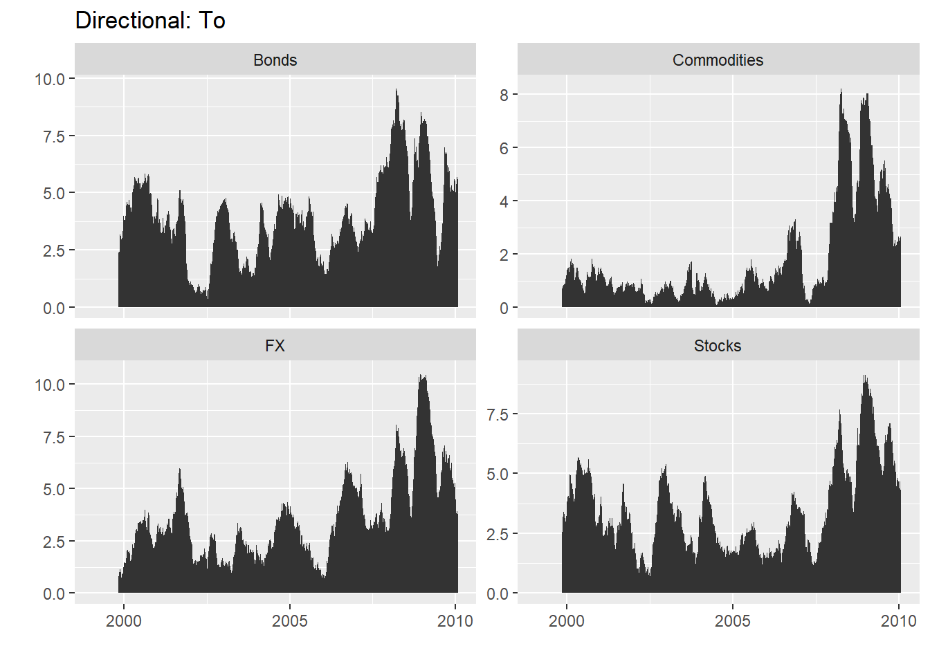
The total volatility spillover appears in the lower right corner of Table, which indicates that, on average, across our entire sample, 12.6% of the volatility forecast error variance in all four markets comes from spillovers

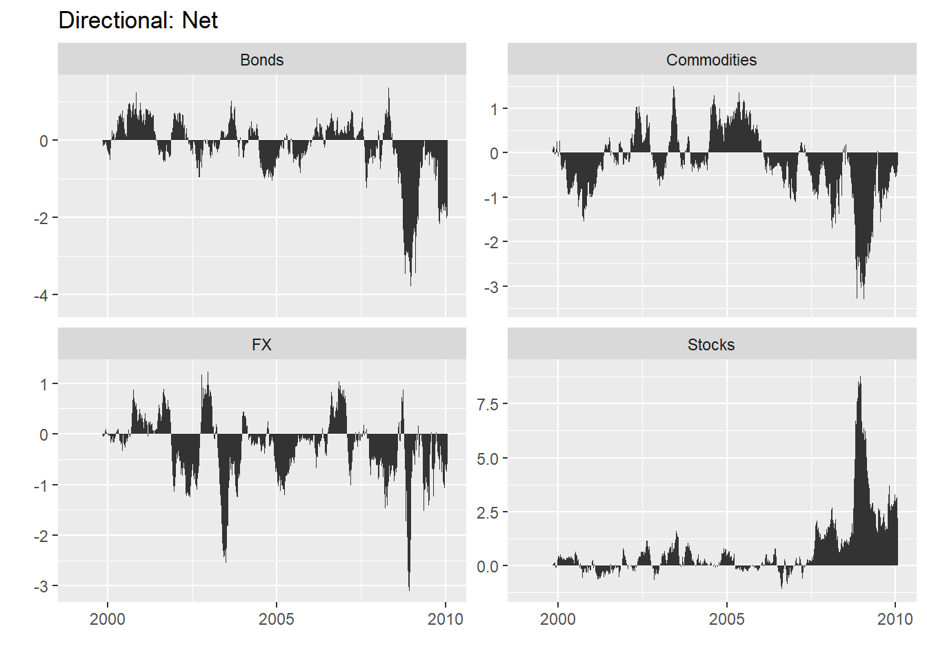
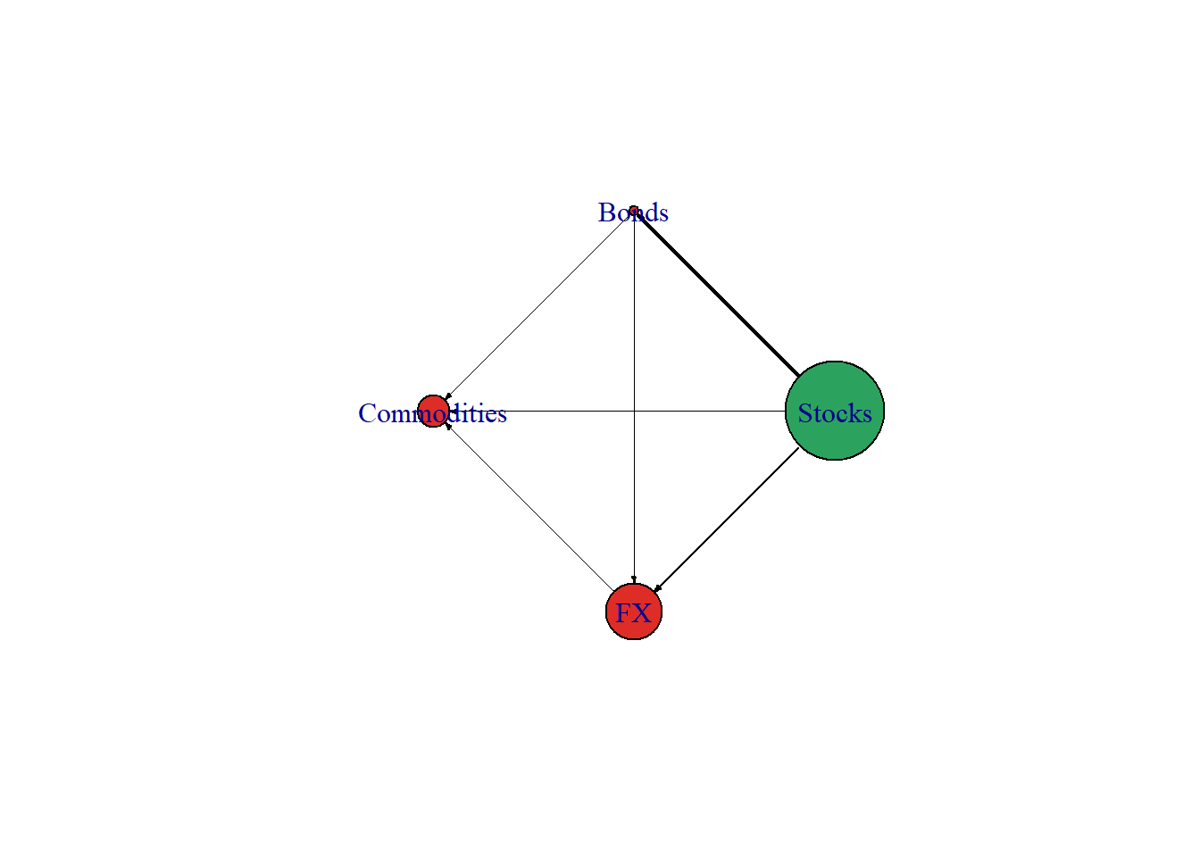
Spillover::net(sp)

Warning in Spillover::net(sp): 'Spillover::net' is deprecated.
Use 'dynamic.spillover' instead.
See help("Deprecated")

                   To      From        Net Transmitter
Stocks      16.373241 11.242998  5.1302430        TRUE
Bonds       18.013154 18.554288 -0.5411342       FALSE
Commodities  4.620061  6.305811 -1.6857500       FALSE
FX          11.361996 14.265355 -2.9033588       FALSE

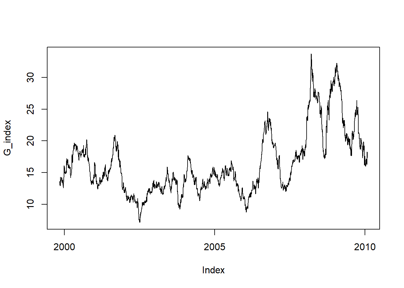
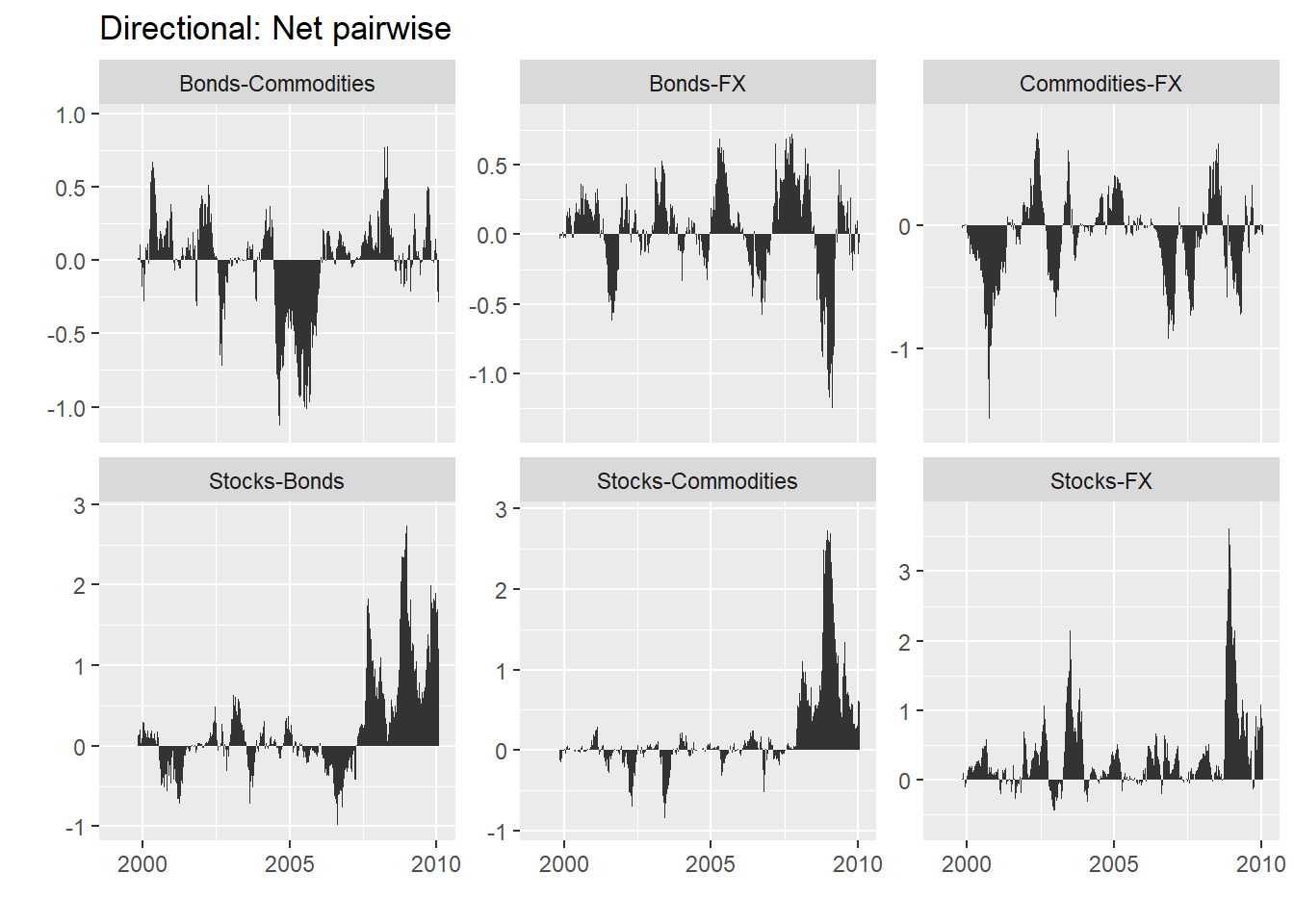
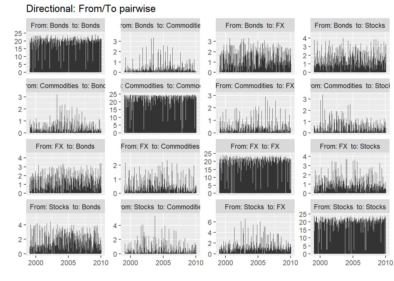
7.5 Dynamic Spillover Index / rolling-sample total volatility spillover

# Data Setting
data(dy2012)
dy2012$Date <- as.Date(dy2012$Date, "%Y-%m-%d")
dy2012 <- as.zoo(dy2012[,-1], order.by = dy2012$Date)
class(dy2012)

[1] "zoo"

# Generalized rolling spillover index based on a VAR(4)
G_index<- total.dynamic.spillover(dy2012, width = 200, index="generalized", p=4) 
head(G_index, n=10)

1999-11-05 1999-11-08 1999-11-09 1999-11-10 1999-11-11 1999-11-12 1999-11-15 
  13.50622   13.60646   13.16968   13.04980   12.95939   12.92011   14.27211 
1999-11-16 1999-11-17 1999-11-18 
  14.04579   13.90963   13.85581 

plot(G_index)

7.6 Directional volatility spillovers

library(zoo)
data(dy2012) # re-import data
class(dy2012)

[1] "data.frame"

dy_results <- dynamic.spillover(dy2012, width=200, remove.own = FALSE)
str(dy_results)

List of 5
 $ from            :'data.frame':   2771 obs. of  5 variables:
  ..$ Date       : Factor w/ 2771 levels "1999-01-25","1999-01-26",..: 1 2 3 4 5 6 7 8 9 10 ...
  ..$ Stocks     : num [1:2771] 0 0 0 0 0 0 0 0 0 0 ...
  ..$ Bonds      : num [1:2771] 0 0 0 0 0 0 0 0 0 0 ...
  ..$ Commodities: num [1:2771] 0 0 0 0 0 0 0 0 0 0 ...
  ..$ FX         : num [1:2771] 0 0 0 0 0 0 0 0 0 0 ...
 $ to              :'data.frame':   2771 obs. of  5 variables:
  ..$ Date       : Factor w/ 2771 levels "1999-01-25","1999-01-26",..: 1 2 3 4 5 6 7 8 9 10 ...
  ..$ Stocks     : num [1:2771] 0 0 0 0 0 0 0 0 0 0 ...
  ..$ Bonds      : num [1:2771] 0 0 0 0 0 0 0 0 0 0 ...
  ..$ Commodities: num [1:2771] 0 0 0 0 0 0 0 0 0 0 ...
  ..$ FX         : num [1:2771] 0 0 0 0 0 0 0 0 0 0 ...
 $ net             :'data.frame':   2771 obs. of  5 variables:
  ..$ Date       : Factor w/ 2771 levels "1999-01-25","1999-01-26",..: 1 2 3 4 5 6 7 8 9 10 ...
  ..$ Stocks     : num [1:2771] 0 0 0 0 0 0 0 0 0 0 ...
  ..$ Bonds      : num [1:2771] 0 0 0 0 0 0 0 0 0 0 ...
  ..$ Commodities: num [1:2771] 0 0 0 0 0 0 0 0 0 0 ...
  ..$ FX         : num [1:2771] 0 0 0 0 0 0 0 0 0 0 ...
 $ net_pairwise    :'data.frame':   2771 obs. of  7 variables:
  ..$ Date              : Factor w/ 2771 levels "1999-01-25","1999-01-26",..: 1 2 3 4 5 6 7 8 9 10 ...
  ..$ Stocks-Bonds      : num [1:2771] 0 0 0 0 0 0 0 0 0 0 ...
  ..$ Stocks-Commodities: num [1:2771] 0 0 0 0 0 0 0 0 0 0 ...
  ..$ Stocks-FX         : num [1:2771] 0 0 0 0 0 0 0 0 0 0 ...
  ..$ Bonds-Commodities : num [1:2771] 0 0 0 0 0 0 0 0 0 0 ...
  ..$ Bonds-FX          : num [1:2771] 0 0 0 0 0 0 0 0 0 0 ...
  ..$ Commodities-FX    : num [1:2771] 0 0 0 0 0 0 0 0 0 0 ...
 $ from_to_pairwise:'data.frame':   44336 obs. of  3 variables:
  ..$ Date     : Factor w/ 2771 levels "1999-01-25","1999-01-26",..: 1 2 3 4 5 6 7 8 9 10 ...
  ..$ variables: chr [1:44336] "From: Stocks  to: Stocks" "From: Stocks  to: Bonds" "From: Stocks  to: Commodities" "From: Stocks  to: FX" ...
  ..$ value    : num [1:44336] 0 0 0 0 0 0 0 0 0 0 ...
 - attr(*, "class")= chr "directional.spillover"

# Directional volatility spillovers, FROM four asset classes.
pp_from <- plotdy(dy_results, direction = "from")

# Directional volatility spillovers, TO four asset classes.
pp_to <- plotdy(dy_results, direction = "to")

# Net volatility spillovers, four asset classes
pp_net <- plotdy(dy_results, direction = "net")

# Net pairwise volatility spillovers
pp_netpairwise <- plotdy(dy_results, direction = "net_pairwise")

pp_from_to_pairwise <- plotdy(dy_results, direction = "from_to_pairwise")

7.7 Connectedness Network

sp <- G.spillover(VAR_4, n.ahead = 10, standardized = F )
datanet <-  Spillover::net(sp)

Warning in Spillover::net(sp): 'Spillover::net' is deprecated.
Use 'dynamic.spillover' instead.
See help("Deprecated")

datanet

                   To      From        Net Transmitter
Stocks      16.373241 11.242998  5.1302430        TRUE
Bonds       18.013154 18.554288 -0.5411342       FALSE
Commodities  4.620061  6.305811 -1.6857500       FALSE
FX          11.361996 14.265355 -2.9033588       FALSE

# Data frame node
node_df <- data.frame(rownames(datanet), rownames(datanet),datanet$Net)
names(node_df) <- c("id","label","size")
head(node_df)

           id       label       size
1      Stocks      Stocks  5.1302430
2       Bonds       Bonds -0.5411342
3 Commodities Commodities -1.6857500
4          FX          FX -2.9033588

sp <- sp[1:4,1:4]
sp

               Stocks     Bonds Commodities        FX
Stocks      88.757002  7.291185   0.3453279  3.606486
Bonds       10.213545 81.445712   2.7269737  5.613770
Commodities  0.468118  3.695953  93.6941893  2.141740
FX           5.691579  7.026017   1.5477592 85.734645

# Data frame edge
m1 <- melt(sp)[melt(upper.tri(sp))$value,] # FROM
m2 <- melt(sp)[melt(lower.tri(sp))$value,] # TO
m1 <- m1[order(m1$X1),]
m2 <- m2[order(m2$X2),]

edge_df <- data.frame("to"=m1[,2],"from"=m1[,1], "weight" = m1$value-m2$value)
library(dplyr)

Attaching package: 'dplyr'

The following object is masked from 'package:reshape':

    rename

The following objects are masked from 'package:igraph':

    as_data_frame, groups, union

The following object is masked from 'package:MASS':

    select

The following objects are masked from 'package:stats':

    filter, lag

The following objects are masked from 'package:base':

    intersect, setdiff, setequal, union

edge_df_positive <- edge_df %>% filter(weight >= 0)
edge_df_negative <- edge_df %>% filter(weight < 0)

edge_df_negative <- edge_df_negative %>%
  mutate(weight = -weight) %>%
  dplyr::rename(to = from, from = to)
edge_df <- bind_rows(edge_df_positive, edge_df_negative)

positive_weight <- edge_df$weight[edge_df$weight > 0]
negative_weight <- edge_df$weight[edge_df$weight < 0]
positive_size <- node_df$size[node_df$size > 0]
negative_size <- node_df$size[node_df$size < 0]

library(RColorBrewer)
Transmitter_color <- "#2ca25f"
else_color <- "#de2d26"
color_vec1 <- ifelse(edge_df$weight > 0, Transmitter_color, else_color)
color_vec2 <- ifelse(node_df$size > 0, Transmitter_color, else_color)

graph <- graph_from_data_frame(edge_df, directed = TRUE, vertices = node_df)
E(graph)$color <- "black" # Egde
V(graph)$color <- color_vec2 # Node
E(graph)$weight <- abs(edge_df$weight)
V(graph)$size <- abs(node_df$size)

E(graph)$weight <- E(graph)$weight / max(E(graph)$weight) * 2
V(graph)$size <- V(graph)$size / max(V(graph)$size) * 50

plot(graph, edge.width = E(graph)$weight, layout=layout_in_circle(graph), edge.arrow.mode=2, edge.arrow.size=0.2)