6  Spatial Regression

6.1 Library

# install.packages("spdep")
# install.packages("spatialreg")
# install.packages("RColorBrewer")
# install.packages("splm")
# install.packages("sf")
# install.packages("ggplot2")
library(spdep)
Warning: package 'spdep' was built under R version 4.4.3
Loading required package: spData
Warning: package 'spData' was built under R version 4.4.3
To access larger datasets in this package, install the spDataLarge
package with: `install.packages('spDataLarge',
repos='https://nowosad.github.io/drat/', type='source')`
Loading required package: sf
Warning: package 'sf' was built under R version 4.4.3
Linking to GEOS 3.13.0, GDAL 3.10.1, PROJ 9.5.1; sf_use_s2() is TRUE
library(spatialreg)
Warning: package 'spatialreg' was built under R version 4.4.3
Loading required package: Matrix

Attaching package: 'spatialreg'
The following objects are masked from 'package:spdep':

    get.ClusterOption, get.coresOption, get.mcOption,
    get.VerboseOption, get.ZeroPolicyOption, set.ClusterOption,
    set.coresOption, set.mcOption, set.VerboseOption,
    set.ZeroPolicyOption
library(RColorBrewer)
library(splm)
Warning: package 'splm' was built under R version 4.4.3
library(sf)
library(ggplot2)
Warning: package 'ggplot2' was built under R version 4.4.3

6.2 Cross-Section

library(readxl)
provinsi <- read_excel("Data/Bab6/provinsi Indonesia.xlsx")
head(provinsi)
# A tibble: 6 × 5
  province    pdrb investment infra revenue
  <chr>      <dbl>      <dbl> <dbl>   <dbl>
1 Aceh     129093.      4485.  0.37  11694.
2 Sumut    571722.     21477.  0.52   8481.
3 Sumbar   179952.      2340.  0.52   4052.
4 Riau     652762.     18957.  0.28   6911.
5 Jambi    155066.      5026.  0.26   3130.
6 Sumsel   331766.     19853.  0.2    5990.

6.2.1 OLS Model

model1 = log(pdrb) ~ log(investment) + log(infra) + log(revenue)
ols = lm(model1, data=provinsi)
summary(ols)

Call:
lm(formula = model1, data = provinsi)

Residuals:
     Min       1Q   Median       3Q      Max 
-0.82306 -0.33812  0.00604  0.32399  0.83581 

Coefficients:
                Estimate Std. Error t value Pr(>|t|)    
(Intercept)      3.95883    0.85379   4.637 6.48e-05 ***
log(investment)  0.42187    0.08375   5.037 2.10e-05 ***
log(infra)       0.24988    0.07807   3.201  0.00323 ** 
log(revenue)     0.53807    0.15207   3.538  0.00133 ** 
---
Signif. codes:  0 '***' 0.001 '**' 0.01 '*' 0.05 '.' 0.1 ' ' 1

Residual standard error: 0.4094 on 30 degrees of freedom
Multiple R-squared:  0.8883,    Adjusted R-squared:  0.8771 
F-statistic: 79.53 on 3 and 30 DF,  p-value: 2.226e-14

6.2.2 Weight Matrix

migrasi <- read_excel("Data/Bab6/matriks migrasi.xlsx", sheet = 2, col_names = FALSE)
New names:
• `` -> `...1`
• `` -> `...2`
• `` -> `...3`
• `` -> `...4`
• `` -> `...5`
• `` -> `...6`
• `` -> `...7`
• `` -> `...8`
• `` -> `...9`
• `` -> `...10`
• `` -> `...11`
• `` -> `...12`
• `` -> `...13`
• `` -> `...14`
• `` -> `...15`
• `` -> `...16`
• `` -> `...17`
• `` -> `...18`
• `` -> `...19`
• `` -> `...20`
• `` -> `...21`
• `` -> `...22`
• `` -> `...23`
• `` -> `...24`
• `` -> `...25`
• `` -> `...26`
• `` -> `...27`
• `` -> `...28`
• `` -> `...29`
• `` -> `...30`
• `` -> `...31`
• `` -> `...32`
• `` -> `...33`
• `` -> `...34`
migrasi = as.matrix(migrasi)
W.migrasi = mat2listw(migrasi)
Warning in mat2listw(migrasi): style is M (missing); style should be set to a
valid value

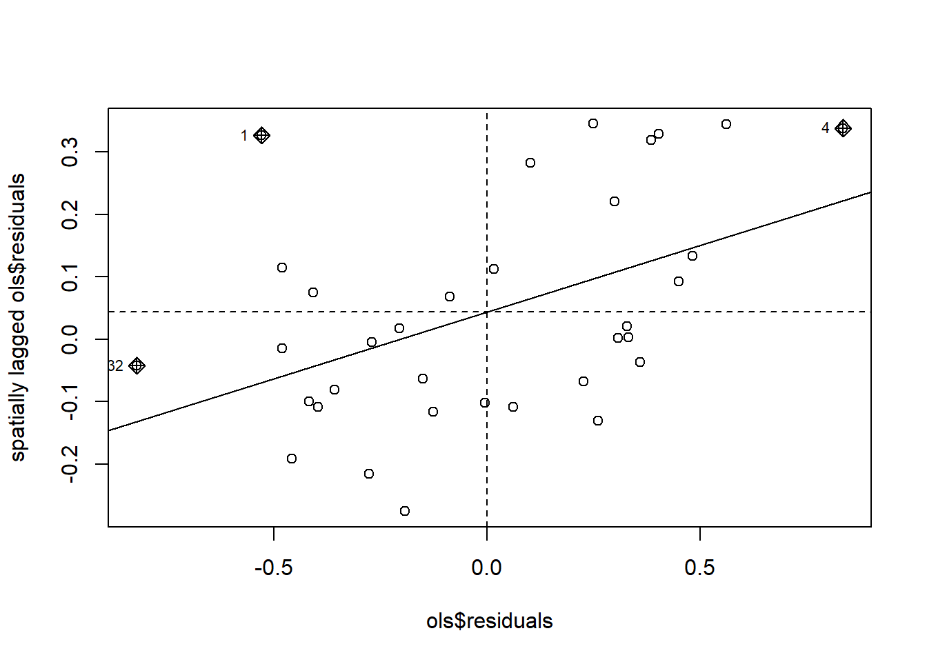
6.2.3 Moran Test and Plot

moran.lm = lm.morantest(ols, W.migrasi)
moran.lm

    Global Moran I for regression residuals

data:  
model: lm(formula = model1, data = provinsi)
weights: W.migrasi

Moran I statistic standard deviate = 3.4669, p-value = 0.0002632
alternative hypothesis: greater
sample estimates:
Observed Moran I      Expectation         Variance 
     0.213239417     -0.048308437      0.005691365 
moran.plot(ols$residuals, W.migrasi)

6.2.4 LM Test

LM = lm.LMtests(ols, W.migrasi, test="all")
Please update scripts to use lm.RStests in place of lm.LMtests
Warning in lm.RStests(model = model, listw = listw, zero.policy = zero.policy,
: Spatial weights matrix not row standardized
LM

    Rao's score (a.k.a Lagrange multiplier) diagnostics for spatial
    dependence

data:  
model: lm(formula = model1, data = provinsi)
test weights: listw

RSerr = 5.4456, df = 1, p-value = 0.01962


    Rao's score (a.k.a Lagrange multiplier) diagnostics for spatial
    dependence

data:  
model: lm(formula = model1, data = provinsi)
test weights: listw

RSlag = 3.2163, df = 1, p-value = 0.07291


    Rao's score (a.k.a Lagrange multiplier) diagnostics for spatial
    dependence

data:  
model: lm(formula = model1, data = provinsi)
test weights: listw

adjRSerr = 3.0702, df = 1, p-value = 0.07974


    Rao's score (a.k.a Lagrange multiplier) diagnostics for spatial
    dependence

data:  
model: lm(formula = model1, data = provinsi)
test weights: listw

adjRSlag = 0.84087, df = 1, p-value = 0.3591


    Rao's score (a.k.a Lagrange multiplier) diagnostics for spatial
    dependence

data:  
model: lm(formula = model1, data = provinsi)
test weights: listw

SARMA = 6.2865, df = 2, p-value = 0.04314

6.2.5 SAR Model

sar.provinsi = lagsarlm(model1, data=provinsi, W.migrasi)
summary(sar.provinsi)

Call:lagsarlm(formula = model1, data = provinsi, listw = W.migrasi)

Residuals:
      Min        1Q    Median        3Q       Max 
-0.679482 -0.291161 -0.083437  0.336403  0.808845 

Type: lag 
Coefficients: (asymptotic standard errors) 
                Estimate Std. Error z value  Pr(>|z|)
(Intercept)     1.744150   1.437574  1.2133 0.2250310
log(investment) 0.380784   0.079364  4.7979 1.603e-06
log(infra)      0.207431   0.073675  2.8155 0.0048701
log(revenue)    0.529174   0.136397  3.8797 0.0001046

Rho: 0.21114, LR test value: 3.0033, p-value: 0.083096
Asymptotic standard error: 0.12002
    z-value: 1.7592, p-value: 0.07854
Wald statistic: 3.0949, p-value: 0.07854

Log likelihood: -14.24739 for lag model
ML residual variance (sigma squared): 0.13454, (sigma: 0.36679)
Number of observations: 34 
Number of parameters estimated: 6 
AIC: 40.495, (AIC for lm: 41.498)
LM test for residual autocorrelation
test value: 2.5558, p-value: 0.10989

6.2.6 Impacts (Spillover)

impacts(sar.provinsi, listw=W.migrasi)
Impact measures (lag, exact):
                   Direct   Indirect     Total
log(investment) 0.3831961 0.09950271 0.4826988
log(infra)      0.2087457 0.05420401 0.2629497
log(revenue)    0.5325268 0.13827873 0.6708055

6.2.7 SEM Model

sem.provinsi = errorsarlm(model1, data=provinsi, W.migrasi)
summary(sem.provinsi)

Call:errorsarlm(formula = model1, data = provinsi, listw = W.migrasi)

Residuals:
      Min        1Q    Median        3Q       Max 
-0.770148 -0.273480 -0.020662  0.325690  0.647156 

Type: error 
Coefficients: (asymptotic standard errors) 
                Estimate Std. Error z value  Pr(>|z|)
(Intercept)     3.831947   0.772493  4.9605 7.031e-07
log(investment) 0.410266   0.072801  5.6354 1.746e-08
log(infra)      0.209178   0.071237  2.9364  0.003321
log(revenue)    0.550807   0.132071  4.1705 3.039e-05

Lambda: 0.60794, LR test value: 5.1345, p-value: 0.023455
Asymptotic standard error: 0.19219
    z-value: 3.1632, p-value: 0.0015604
Wald statistic: 10.006, p-value: 0.0015604

Log likelihood: -13.18178 for error model
ML residual variance (sigma squared): 0.11956, (sigma: 0.34577)
Number of observations: 34 
Number of parameters estimated: 6 
AIC: 38.364, (AIC for lm: 41.498)

6.3 Spatial Panel

library(readxl)
paneljateng <- read_excel("Data/Bab6/panel jateng.xlsx")
head(paneljateng)
# A tibble: 6 × 8
  Region        Tahun      PDRB     AK     PAD      UMK   IPM NO   
  <chr>         <dbl>     <dbl>  <dbl>   <dbl>    <dbl> <dbl> <chr>
1 Kab. Cilacap   2011 78156819. 797518 173141.  718667.  64.7 01   
2 Kab. Cilacap   2012 79702238. 716465 196673.  773000   65.7 01   
3 Kab. Cilacap   2013 81022670. 729059 278508.  887667   66.8 01   
4 Kab. Cilacap   2014 83392999. 736247 373907. 1016667.  67.2 01   
5 Kab. Cilacap   2015 88777805. 715819 409846. 1195667.  67.8 01   
6 Kab. Banyumas  2011 24538596. 761034 193263.  750000   67.4 02   

6.3.1 Static Panel Regression

library(plm)
modelpanel = log(PDRB) ~ log(AK) + log(PAD) + log(UMK) + log(IPM)
fem1 = plm(modelpanel, data=paneljateng, index=c("Region", "Tahun"), model="within")
rem1 = plm(modelpanel, data=paneljateng, index=c("Region", "Tahun"), model="random")
phtest(fem1, rem1)

    Hausman Test

data:  modelpanel
chisq = 37.156, df = 4, p-value = 1.673e-07
alternative hypothesis: one model is inconsistent
library(lmtest)
Loading required package: zoo

Attaching package: 'zoo'
The following objects are masked from 'package:base':

    as.Date, as.Date.numeric
bptest(fem1)

    studentized Breusch-Pagan test

data:  fem1
BP = 5.8081, df = 4, p-value = 0.2139
pbgtest(fem1)

    Breusch-Godfrey/Wooldridge test for serial correlation in panel models

data:  modelpanel
chisq = 51.619, df = 5, p-value = 6.458e-10
alternative hypothesis: serial correlation in idiosyncratic errors

6.3.2 Depndency Test

pcdtest(fem1, test="lm")

    Breusch-Pagan LM test for cross-sectional dependence in panels

data:  log(PDRB) ~ log(AK) + log(PAD) + log(UMK) + log(IPM)
chisq = 1268.3, df = 595, p-value < 2.2e-16
alternative hypothesis: cross-sectional dependence
pcdtest(fem1, test="cd")

    Pesaran CD test for cross-sectional dependence in panels

data:  log(PDRB) ~ log(AK) + log(PAD) + log(UMK) + log(IPM)
z = 12.724, p-value < 2.2e-16
alternative hypothesis: cross-sectional dependence

6.3.3 Maps Visualization

jateng.map = st_read('Data/Bab6/peta jateng/Jawa_Tengah.shp')
Reading layer `Jawa_Tengah' from data source 
  `D:\Dokumentasi\econometricsbook\Data\Bab6\peta jateng\Jawa_Tengah.shp' 
  using driver `ESRI Shapefile'
Simple feature collection with 35 features and 4 fields
Geometry type: MULTIPOLYGON
Dimension:     XY
Bounding box:  xmin: 108.5559 ymin: -8.211962 xmax: 111.6914 ymax: -5.725698
Geodetic CRS:  WGS 84
jateng2011 = subset(paneljateng,(Tahun==2011))
jateng2011 = merge(jateng.map, jateng2011, by.x="KABKOTNO", by.y="NO")
jateng2011 <- st_make_valid(jateng2011)
ggplot(jateng2011) +
  geom_sf(aes(fill = PDRB)) +
  scale_fill_gradientn(colours = brewer.pal(5, "Blues"),
                       values = scales::rescale(seq(min(jateng2011$PDRB), 
                                                    max(jateng2011$PDRB)*1.01, 
                                                    length = 6))) +
  theme_minimal() +
  labs(fill = "PDRB")

ggplot(jateng2011) +
  geom_sf(aes(fill = IPM)) +
  scale_fill_gradientn(colours = brewer.pal(5, "Greens"),
                       values = scales::rescale(seq(min(jateng2011$IPM), 
                                                    max(jateng2011$IPM)*1.01, 
                                                    length = 6))) +
  theme_minimal() +
  labs(fill = "IPM")

6.3.4 Function for Spatial Panel Evalutation

godf.spml<-function(object, k=2, criterion=c("AIC", "BIC"),  ...){
  s<-summary(object)
  l<-s$logLik
  np<- length(coef(s))
  N<- nrow(s$model)
  if(criterion=="AIC"){
    aic<- -2*l+k*np
    names(aic)<-"AIC"
    return(aic)
  }
  if(criterion=="BIC"){
    bic<- -2*l+log(N)*np
    names(bic)<-"BIC"
    if(k!=2){
      warning("parameter <k> not used for BIC")
    }
    return(bic)
  }
}

6.3.5 Spatial Panel Model with Contiguity Weight Matrix

jateng.map <- st_make_valid(jateng.map)
listqueen = poly2nb(jateng.map, queen=TRUE)
W.queen = nb2listw(listqueen, style="W")
W.queen
Characteristics of weights list object:
Neighbour list object:
Number of regions: 35 
Number of nonzero links: 148 
Percentage nonzero weights: 12.08163 
Average number of links: 4.228571 

Weights style: W 
Weights constants summary:
   n   nn S0       S1       S2
W 35 1225 35 18.64242 151.0178
# SAR Model
sar.fem.contig = spml(modelpanel, data=paneljateng, listw=W.queen, model="within", lag=TRUE, spatial.error="none")
sar.rem.contig = spml(modelpanel, data=paneljateng, listw=W.queen, model="random", lag=TRUE, spatial.error="none")
sphtest(sar.fem.contig, sar.rem.contig)

    Hausman test for spatial models

data:  modelpanel
chisq = 0.15855, df = 4, p-value = 0.997
alternative hypothesis: one model is inconsistent
godf.spml(sar.rem.contig, criterion="AIC")
      AIC 
-703.0118 
# SEM Model
sem.fem.contig = spml(modelpanel, data=paneljateng, listw=W.queen, model="within", lag=FALSE, spatial.error="b")
sem.rem.contig = spml(modelpanel, data=paneljateng, listw=W.queen, model="random", lag=FALSE, spatial.error="b")
sphtest(sem.fem.contig, sem.rem.contig)

    Hausman test for spatial models

data:  modelpanel
chisq = 5.4546, df = 4, p-value = 0.2438
alternative hypothesis: one model is inconsistent
godf.spml(sem.rem.contig, criterion="AIC")
      AIC 
-633.5611 

6.3.6 Spatial Panel Model with KNN Weight Matrix

# K-nearest neighbour with 5 neighbour 
centroids <- st_centroid(jateng.map)
Warning: st_centroid assumes attributes are constant over geometries
coords <- st_coordinates(centroids)
neighbour = knearneigh(coords, k=5, longlat=T) 
neighbourlist = knn2nb(neighbour)                              
mat.knn5 = nb2mat(neighbourlist, style="W")                     
W.knn5 = nb2listw(neighbourlist, style="W")
W.knn5
Characteristics of weights list object:
Neighbour list object:
Number of regions: 35 
Number of nonzero links: 175 
Percentage nonzero weights: 14.28571 
Average number of links: 5 
Non-symmetric neighbours list

Weights style: W 
Weights constants summary:
   n   nn S0    S1     S2
W 35 1225 35 12.44 144.48
# SAR Model
sar.fem.5nn = spml(modelpanel, data=paneljateng, listw=W.knn5, model="within", lag=TRUE, spatial.error="none")
sar.rem.5nn = spml(modelpanel, data=paneljateng, listw=W.knn5, model="random", lag=TRUE, spatial.error="none")
sphtest(sar.fem.5nn, sar.rem.5nn)

    Hausman test for spatial models

data:  modelpanel
chisq = 0.9208, df = 4, p-value = 0.9216
alternative hypothesis: one model is inconsistent
godf.spml(sar.rem.5nn, criterion="AIC")
      AIC 
-717.8954 
# SEM Model
sem.fem.5nn = spml(modelpanel, data=paneljateng, listw=W.knn5, model="within", lag=FALSE, spatial.error="b")
sem.rem.5nn = spml(modelpanel, data=paneljateng, listw=W.knn5, model="random", lag=FALSE, spatial.error="b")
sphtest(sem.fem.5nn, sem.rem.5nn)

    Hausman test for spatial models

data:  modelpanel
chisq = 5.3246, df = 4, p-value = 0.2556
alternative hypothesis: one model is inconsistent
godf.spml(sem.rem.5nn, criterion="AIC")
      AIC 
-636.4432 

6.3.7 Best Model

summary(sar.rem.5nn)
ML panel with spatial lag, random effects 

Call:
spreml(formula = formula, data = data, index = index, w = listw2mat(listw), 
    w2 = listw2mat(listw2), lag = lag, errors = errors, cl = cl)

Residuals:
   Min. 1st Qu.  Median    Mean 3rd Qu.    Max. 
   11.2    12.1    12.4    12.4    12.7    14.2 

Error variance parameters:
    Estimate Std. Error t-value  Pr(>|t|)    
phi   4204.2     1172.1  3.5868 0.0003348 ***

Spatial autoregressive coefficient:
       Estimate Std. Error t-value  Pr(>|t|)    
lambda 0.750456   0.053423  14.047 < 2.2e-16 ***

Coefficients:
             Estimate Std. Error t-value Pr(>|t|)   
(Intercept) 1.2042585  0.7177210  1.6779 0.093368 . 
log(AK)     0.0474276  0.0241591  1.9631 0.049630 * 
log(PAD)    0.0134898  0.0063019  2.1406 0.032306 * 
log(UMK)    0.0470068  0.0167872  2.8002 0.005108 **
log(IPM)    0.3633197  0.1772088  2.0502 0.040342 * 
---
Signif. codes:  0 '***' 0.001 '**' 0.01 '*' 0.05 '.' 0.1 ' ' 1

6.3.8 Impacts (Spillovr) - Only for SAR Model

# Direct and Indirect Effect
time = length(unique(paneljateng$Tahun))
sW.5knn = kronecker(Diagonal(time), listw2dgCMatrix(W.knn5))
set.seed(12345)
trMatc = trW(sW.5knn, type="mult")
imp = impacts(sar.rem.5nn, tr = trMatc, R = 200)
summary(imp, zstats=TRUE, short=T)
Impact measures (lag, trace):
             Direct  Indirect      Total
log(AK)  0.05723256 0.1327900 0.19002256
log(PAD) 0.01627868 0.0377695 0.05404818
log(UMK) 0.05672481 0.1316119 0.18833673
log(IPM) 0.43843072 1.0172393 1.45567006
========================================================
Simulation results ( variance matrix):
========================================================
Simulated standard errors
              Direct   Indirect      Total
log(AK)  0.029013340 0.08364084 0.10974771
log(PAD) 0.007350001 0.02062333 0.02706877
log(UMK) 0.021472770 0.08001914 0.09849884
log(IPM) 0.228933484 0.65969232 0.86740920

Simulated z-values:
           Direct Indirect    Total
log(AK)  1.994004 1.692971 1.817389
log(PAD) 2.422582 2.079346 2.242031
log(UMK) 2.675263 1.800226 2.045687
log(IPM) 1.772324 1.503129 1.610943

Simulated p-values:
         Direct    Indirect Total   
log(AK)  0.0461516 0.090461 0.069158
log(PAD) 0.0154107 0.037586 0.024959
log(UMK) 0.0074671 0.071825 0.040787
log(IPM) 0.0763407 0.132806 0.107192