3  Univariate Time Series

3.1 Data EDA

library(readxl)
hargaberas <- read_excel("Data/Bab 3/ARIMA.xlsx")
hargaberas = hargaberas[,c(-1)]
hargaberas = ts(hargaberas, start=c(2012,1), frequency=12)
hargaberas

       Jan   Feb   Mar   Apr   May   Jun   Jul   Aug   Sep   Oct   Nov   Dec
2012  8726  8778  8687  8583  8537  8554  8606  8635  8624  8624  8655  8702
2013  8835  8843  8783  8711  8681  8784  9018  9057  9058  9108  9152  9262
2014  9433  9531  9596  9425  9414  9462  9525  9525  9694  9781  9924 10344
2015 10612 10766 10987 10648 10569 10679 10732 10935 11055 11169 11365 11465
2016 11614 11729 11678 11449 11417 11469 11498 11475 11448 11433 11450 11476
2017 11579 11571 11494 11449 11465 11465 11448 11411 11482 11552 11665 11838
2018 12276 12414 12299 12035 11943 11907 11936 11899 11900 11926 12013 12106

plot(hargaberas, main="Harga Beras di Perdagangan Besar")

dekomposisi = decompose(hargaberas)
plot(dekomposisi)

3.2 ACF and PACF Plot

# plot acf dan pacf
acf(hargaberas, lag=48)

pacf(hargaberas, lag=48)

##Stationary Test

library(aTSA)

Attaching package: 'aTSA'

The following object is masked from 'package:graphics':

    identify

# Augmented Dickey-Fuller Test 
adf.test(hargaberas)

Augmented Dickey-Fuller Test 
alternative: stationary 
 
Type 1: no drift no trend 
     lag  ADF p.value
[1,]   0 2.96   0.990
[2,]   1 1.65   0.975
[3,]   2 2.04   0.990
[4,]   3 2.18   0.990
Type 2: with drift no trend 
     lag    ADF p.value
[1,]   0 -0.537   0.858
[2,]   1 -0.717   0.795
[3,]   2 -0.831   0.755
[4,]   3 -0.917   0.724
Type 3: with drift and trend 
     lag   ADF p.value
[1,]   0 -1.42   0.814
[2,]   1 -2.56   0.340
[3,]   2 -2.00   0.570
[4,]   3 -1.78   0.663
---- 
Note: in fact, p.value = 0.01 means p.value <= 0.01 

# Firs Difference Form
adf.test(diff(hargaberas))

Augmented Dickey-Fuller Test 
alternative: stationary 
 
Type 1: no drift no trend 
     lag   ADF p.value
[1,]   0 -5.11    0.01
[2,]   1 -5.02    0.01
[3,]   2 -4.42    0.01
[4,]   3 -4.36    0.01
Type 2: with drift no trend 
     lag   ADF p.value
[1,]   0 -5.47    0.01
[2,]   1 -5.58    0.01
[3,]   2 -5.10    0.01
[4,]   3 -5.27    0.01
Type 3: with drift and trend 
     lag   ADF p.value
[1,]   0 -5.43    0.01
[2,]   1 -5.55    0.01
[3,]   2 -5.10    0.01
[4,]   3 -5.28    0.01
---- 
Note: in fact, p.value = 0.01 means p.value <= 0.01 

3.3 ARIMA

library(forecast)

Registered S3 method overwritten by 'quantmod':
  method            from
  as.zoo.data.frame zoo 

Attaching package: 'forecast'

The following object is masked from 'package:aTSA':

    forecast

auto.arima(hargaberas, trace=TRUE)

 ARIMA(2,1,2)(1,1,1)[12]                    : Inf
 ARIMA(0,1,0)(0,1,0)[12]                    : 884.0934
 ARIMA(1,1,0)(1,1,0)[12]                    : 872.3993
 ARIMA(0,1,1)(0,1,1)[12]                    : Inf
 ARIMA(1,1,0)(0,1,0)[12]                    : 876.5573
 ARIMA(1,1,0)(2,1,0)[12]                    : 863.6643
 ARIMA(1,1,0)(2,1,1)[12]                    : Inf
 ARIMA(1,1,0)(1,1,1)[12]                    : Inf
 ARIMA(0,1,0)(2,1,0)[12]                    : 867.3178
 ARIMA(2,1,0)(2,1,0)[12]                    : 865.871
 ARIMA(1,1,1)(2,1,0)[12]                    : 865.1084
 ARIMA(0,1,1)(2,1,0)[12]                    : 862.9856
 ARIMA(0,1,1)(1,1,0)[12]                    : 871.9363
 ARIMA(0,1,1)(2,1,1)[12]                    : Inf
 ARIMA(0,1,1)(1,1,1)[12]                    : Inf
 ARIMA(0,1,2)(2,1,0)[12]                    : 861.8543
 ARIMA(0,1,2)(1,1,0)[12]                    : 872.2305
 ARIMA(0,1,2)(2,1,1)[12]                    : Inf
 ARIMA(0,1,2)(1,1,1)[12]                    : Inf
 ARIMA(1,1,2)(2,1,0)[12]                    : 867.0498
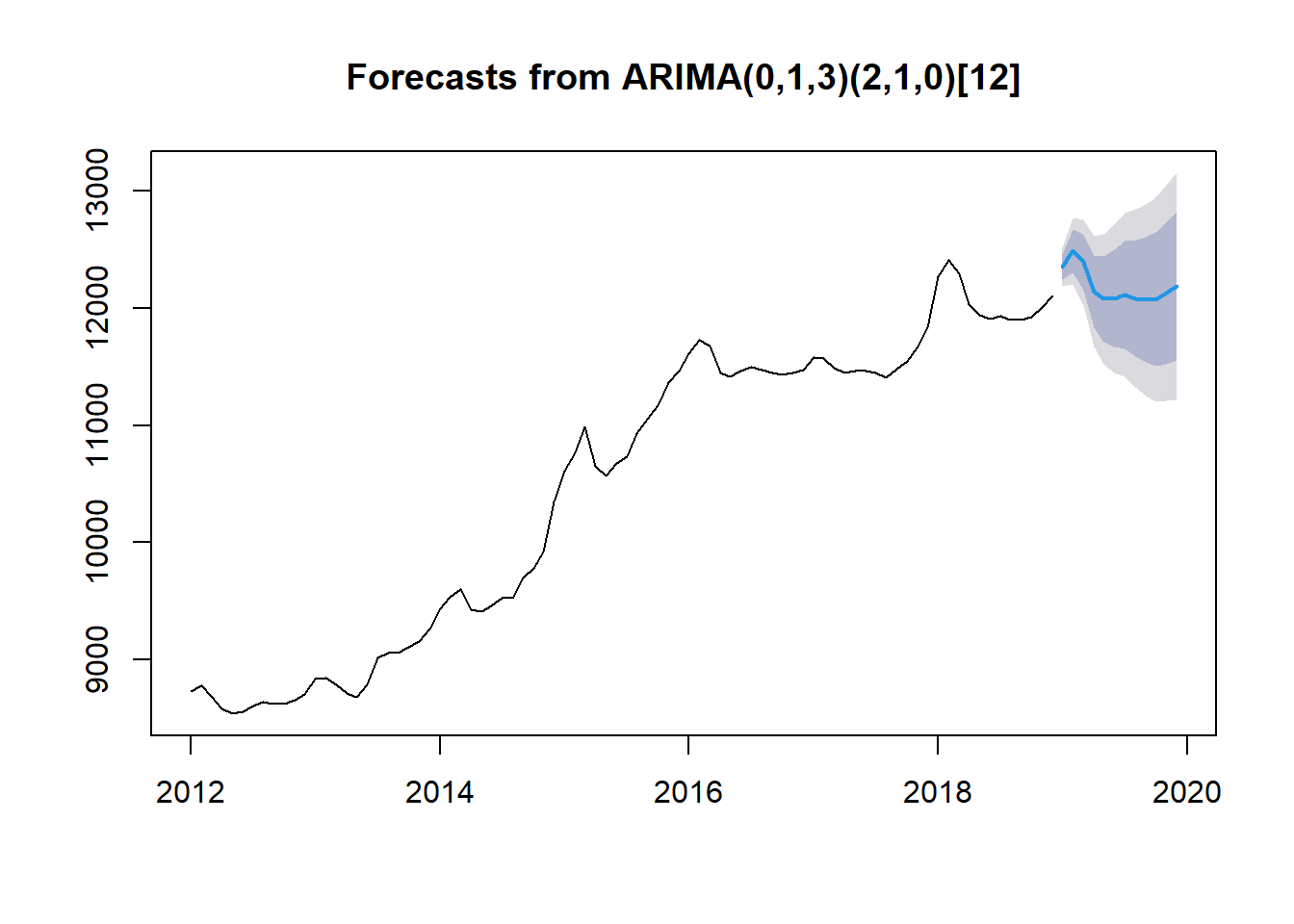
 ARIMA(0,1,3)(2,1,0)[12]                    : 854.8026
 ARIMA(0,1,3)(1,1,0)[12]                    : 865.2557
 ARIMA(0,1,3)(2,1,1)[12]                    : Inf
 ARIMA(0,1,3)(1,1,1)[12]                    : Inf
 ARIMA(1,1,3)(2,1,0)[12]                    : Inf
 ARIMA(0,1,4)(2,1,0)[12]                    : 857.2177
 ARIMA(1,1,4)(2,1,0)[12]                    : 859.7882

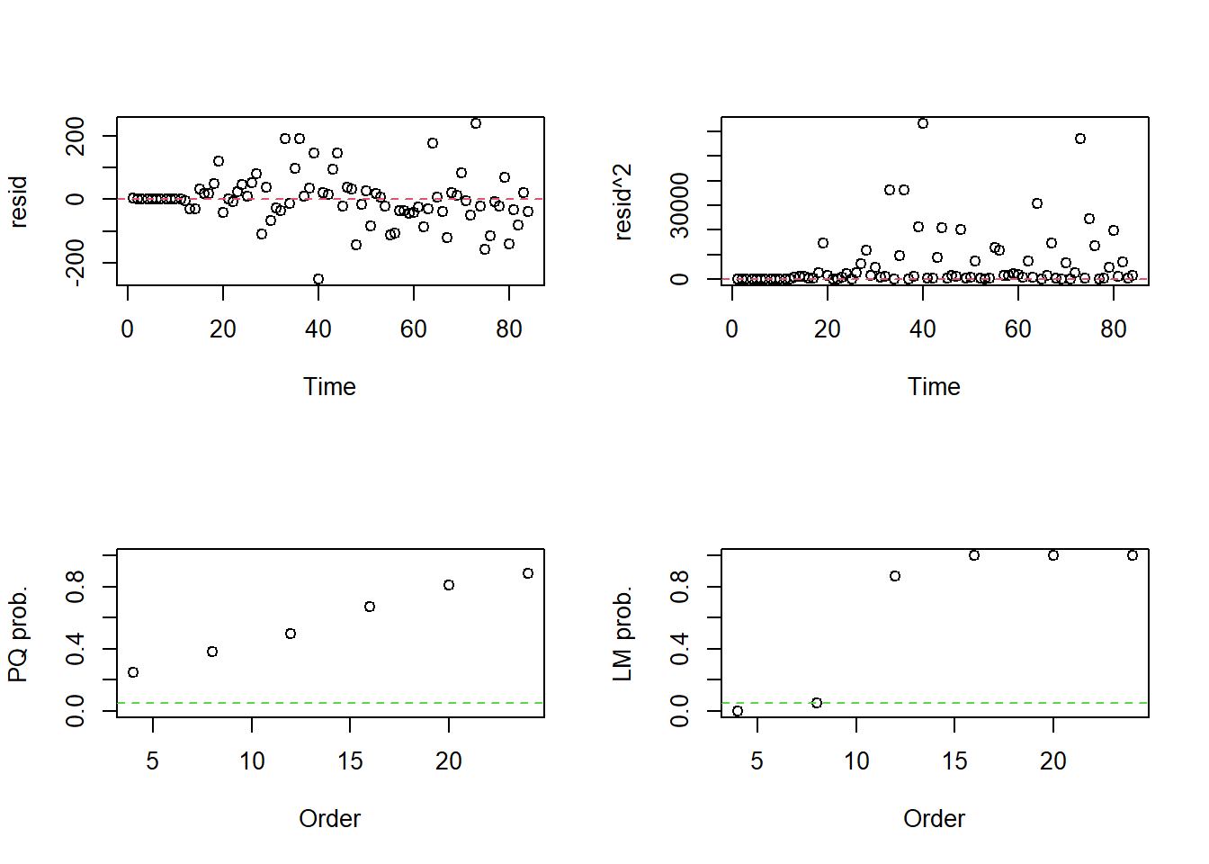
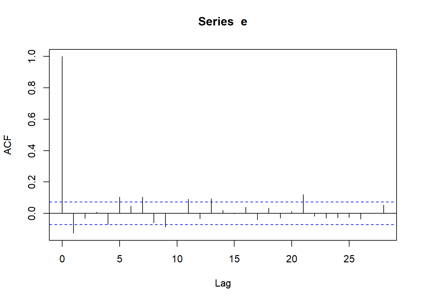
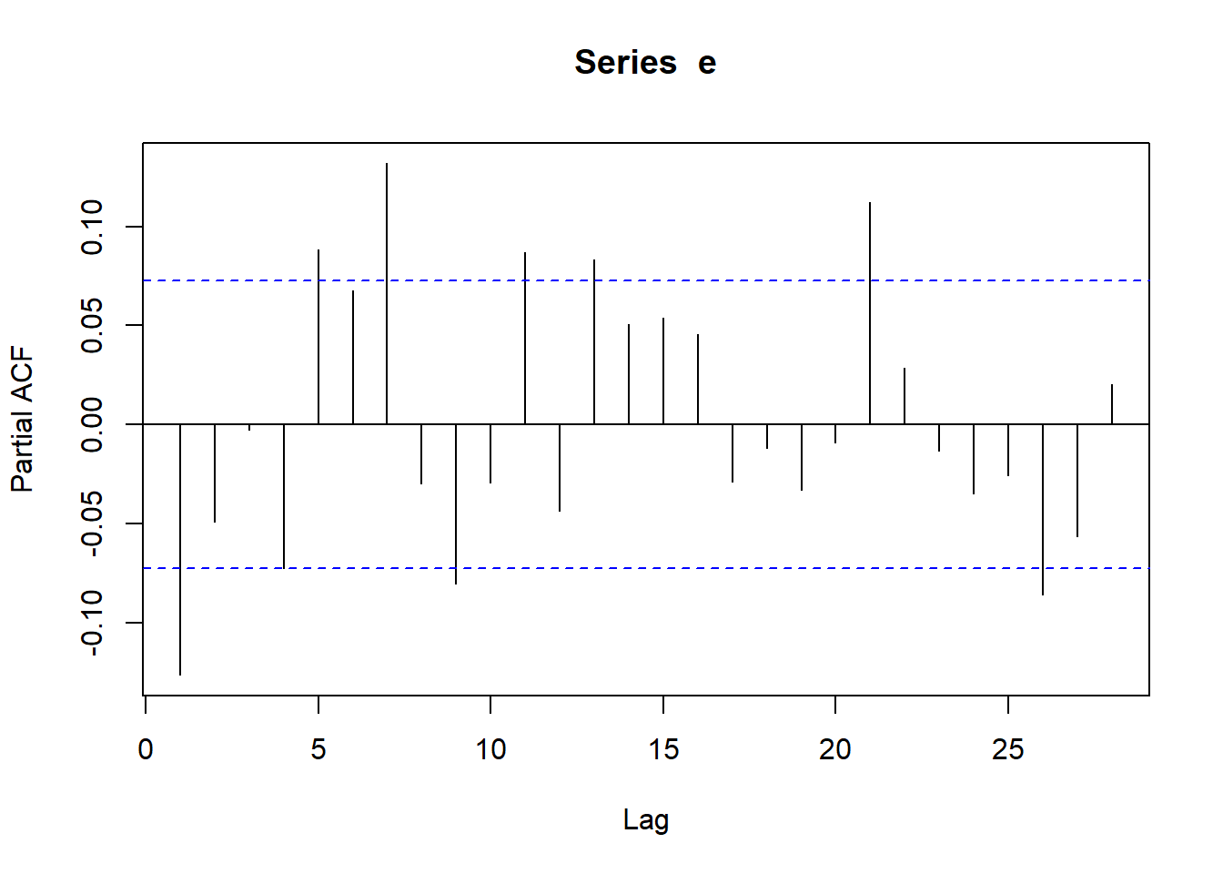
 Best model: ARIMA(0,1,3)(2,1,0)[12]                    

Series: hargaberas 
ARIMA(0,1,3)(2,1,0)[12] 

Coefficients:
         ma1     ma2     ma3     sar1     sar2
      0.3775  0.0028  0.4180  -0.4831  -0.4956
s.e.  0.1166  0.1301  0.1403   0.1231   0.1239

sigma^2 = 7757:  log likelihood = -420.75
AIC=853.49   AICc=854.8   BIC=867.07

library(lmtest)

Loading required package: zoo

Attaching package: 'zoo'

The following objects are masked from 'package:base':

    as.Date, as.Date.numeric

# Best model: ARIMA(0,1,3)(2,1,0)[12]
model1 = arima(hargaberas, order=c(0,1,3), seasonal=list(order=c(2,1,0), period=12))
coeftest(model1)

z test of coefficients:

      Estimate Std. Error z value  Pr(>|z|)    
ma1   0.377526   0.116627  3.2370  0.001208 ** 
ma2   0.002799   0.130115  0.0215  0.982837    
ma3   0.417985   0.140264  2.9800  0.002883 ** 
sar1 -0.483126   0.123055 -3.9261 8.634e-05 ***
sar2 -0.495630   0.123883 -4.0008 6.313e-05 ***
---
Signif. codes:  0 '***' 0.001 '**' 0.01 '*' 0.05 '.' 0.1 ' ' 1

# Arch Test
arch.test(model1)

ARCH heteroscedasticity test for residuals 
alternative: heteroscedastic 

Portmanteau-Q test: 
     order    PQ p.value
[1,]     4  5.41   0.247
[2,]     8  8.53   0.384
[3,]    12 11.36   0.498
[4,]    16 13.03   0.670
[5,]    20 14.44   0.808
[6,]    24 16.04   0.887
Lagrange-Multiplier test: 
     order    LM  p.value
[1,]     4 41.16 6.04e-09
[2,]     8 13.84 5.42e-02
[3,]    12  6.06 8.69e-01
[4,]    16  3.39 9.99e-01
[5,]    20  2.16 1.00e+00
[6,]    24  1.16 1.00e+00

# Autocorrelartion Test
Box.test(model1$residuals, lag = 1, type = c("Ljung-Box"), fitdf = 0)

    Box-Ljung test

data:  model1$residuals
X-squared = 0.0041444, df = 1, p-value = 0.9487

# Forecasting
forecast(model1, h=12)

         Point Forecast    Lo 80    Hi 80    Lo 95    Hi 95
Jan 2019       12355.67 12246.95 12464.39 12189.39 12521.95
Feb 2019       12493.09 12308.02 12678.16 12210.05 12776.13
Mar 2019       12392.80 12154.53 12631.07 12028.40 12757.21
Apr 2019       12143.41 11835.19 12451.63 11672.03 12614.80
May 2019       12079.80 11714.79 12444.80 11521.57 12638.02
Jun 2019       12086.96 11672.89 12501.04 11453.70 12720.23
Jul 2019       12116.54 11658.63 12574.45 11416.22 12816.85
Aug 2019       12086.48 11588.57 12584.38 11325.00 12847.96
Sep 2019       12072.73 11537.81 12607.64 11254.64 12890.81
Oct 2019       12077.85 11508.32 12647.38 11206.83 12948.88
Nov 2019       12129.83 11527.68 12731.99 11208.92 13050.75
Dec 2019       12188.63 11555.52 12821.73 11220.38 13156.88

plot(forecast(model1, h=12))

3.4 ARCH-GARCH

library(readxl)
kurs <- read_excel("Data/Bab 3/ARCH-GARCH.xlsx")
kurs = kurs[,c(-1)]
Dates = seq(as.Date("2019-01-01"), as.Date("2020-12-31"), "day") 

library(xts)
kurs = xts(kurs, order.by = Dates)
plot(kurs, main="Nilai Tukar US Dollar terhadap Rupiah")

# ARIMA
auto.arima(kurs, trace=TRUE)

 Fitting models using approximations to speed things up...

 ARIMA(2,1,2) with drift         : 8738.664
 ARIMA(0,1,0) with drift         : 8755.631
 ARIMA(1,1,0) with drift         : 8745.702
 ARIMA(0,1,1) with drift         : 8744.836
 ARIMA(0,1,0)                    : 8753.644
 ARIMA(1,1,2) with drift         : 8742.017
 ARIMA(2,1,1) with drift         : 8748.12
 ARIMA(3,1,2) with drift         : 8746.649
 ARIMA(2,1,3) with drift         : 8740.697
 ARIMA(1,1,1) with drift         : 8746.629
 ARIMA(1,1,3) with drift         : 8743.813
 ARIMA(3,1,1) with drift         : 8748.657
 ARIMA(3,1,3) with drift         : 8751.34
 ARIMA(2,1,2)                    : 8736.651
 ARIMA(1,1,2)                    : 8740.011
 ARIMA(2,1,1)                    : 8746.122
 ARIMA(3,1,2)                    : 8744.611
 ARIMA(2,1,3)                    : 8738.68
 ARIMA(1,1,1)                    : 8744.657
 ARIMA(1,1,3)                    : 8741.802
 ARIMA(3,1,1)                    : 8746.636
 ARIMA(3,1,3)                    : 8749.317

 Now re-fitting the best model(s) without approximations...

 ARIMA(2,1,2)                    : 8739.165

 Best model: ARIMA(2,1,2)                    

Series: kurs 
ARIMA(2,1,2) 

Coefficients:
         ar1      ar2      ma1     ma2
      1.2304  -0.7997  -1.3560  0.8726
s.e.  0.0650   0.0506   0.0599  0.0425

sigma^2 = 9181:  log likelihood = -4364.54
AIC=8739.08   AICc=8739.16   BIC=8762.05

#  Best model: ARIMA(2,1,2)
model2 = arima(kurs, order=c(2,1,2))
coeftest(model2)

z test of coefficients:

     Estimate Std. Error z value  Pr(>|z|)    
ar1  1.230421   0.065027  18.922 < 2.2e-16 ***
ar2 -0.799713   0.050577 -15.812 < 2.2e-16 ***
ma1 -1.355960   0.059905 -22.635 < 2.2e-16 ***
ma2  0.872641   0.042457  20.554 < 2.2e-16 ***
---
Signif. codes:  0 '***' 0.001 '**' 0.01 '*' 0.05 '.' 0.1 ' ' 1

# ARCH Test
arch.test(model2)

ARCH heteroscedasticity test for residuals 
alternative: heteroscedastic 

Portmanteau-Q test: 
     order    PQ p.value
[1,]     4  70.7 1.6e-14
[2,]     8 134.2 0.0e+00
[3,]    12 188.4 0.0e+00
[4,]    16 206.3 0.0e+00
[5,]    20 216.8 0.0e+00
[6,]    24 225.0 0.0e+00
Lagrange-Multiplier test: 
     order   LM  p.value
[1,]     4 1471 0.00e+00
[2,]     8  446 0.00e+00
[3,]    12  251 0.00e+00
[4,]    16  179 0.00e+00
[5,]    20  135 0.00e+00
[6,]    24  106 1.14e-12

if p.value <- 0.05 = ARCH/GARCH

library(fGarch)

Warning: package 'fGarch' was built under R version 4.4.3

NOTE: Packages 'fBasics', 'timeDate', and 'timeSeries' are no longer
attached to the search() path when 'fGarch' is attached.

If needed attach them yourself in your R script by e.g.,
        require("timeSeries")

# Stationary Test
# Phillips-Perron Unit Root Test 
pp.test(kurs)

Phillips-Perron Unit Root Test 
alternative: stationary 
 
Type 1: no drift no trend 
 lag   Z_rho p.value
   6 -0.0408   0.683
----- 
 Type 2: with drift no trend 
 lag Z_rho p.value
   6 -11.1   0.107
----- 
 Type 3: with drift and trend 
 lag Z_rho p.value
   6 -12.1   0.367
--------------- 
Note: p-value = 0.01 means p.value <= 0.01 

pp.test(diff(kurs))

Phillips-Perron Unit Root Test 
alternative: stationary 
 
Type 1: no drift no trend 
 lag Z_rho p.value
   6  -804    0.01
----- 
 Type 2: with drift no trend 
 lag Z_rho p.value
   6  -804    0.01
----- 
 Type 3: with drift and trend 
 lag Z_rho p.value
   6  -804    0.01
--------------- 
Note: p-value = 0.01 means p.value <= 0.01 

e = diff(kurs)[-1]
par(mfrow=c(1,1))
acf(e)

pacf(e)

plot(e)

# ARCH(1) = GARCH(1,0)
model10 = garchFit(~garch(1,0), data=e, trace=FALSE)
summary(model10)

Title:
 GARCH Modelling 

Call:
 garchFit(formula = ~garch(1, 0), data = e, trace = FALSE) 

Mean and Variance Equation:
 data ~ garch(1, 0)
<environment: 0x000001e4fdd103c0>
 [data = e]

Conditional Distribution:
 norm 

Coefficient(s):
        mu       omega      alpha1  
  -1.15887  5442.67260     0.61303  

Std. Errors:
 based on Hessian 

Error Analysis:
        Estimate  Std. Error  t value Pr(>|t|)    
mu       -1.1589      2.8293   -0.410    0.682    
omega  5442.6726    374.5058   14.533  < 2e-16 ***
alpha1    0.6130      0.1073    5.713 1.11e-08 ***
---
Signif. codes:  0 '***' 0.001 '**' 0.01 '*' 0.05 '.' 0.1 ' ' 1

Log Likelihood:
 -4303.768    normalized:  -5.895573 

Description:
 Sat Jul  5 23:34:33 2025 by user: derik 


Standardised Residuals Tests:
                                  Statistic      p-Value
 Jarque-Bera Test   R    Chi^2  4839.704460 0.000000e+00
 Shapiro-Wilk Test  R    W         0.839958 0.000000e+00
 Ljung-Box Test     R    Q(10)    29.630084 9.844469e-04
 Ljung-Box Test     R    Q(15)    39.676117 5.074432e-04
 Ljung-Box Test     R    Q(20)    41.959542 2.799349e-03
 Ljung-Box Test     R^2  Q(10)    91.109411 3.219647e-15
 Ljung-Box Test     R^2  Q(15)   147.246211 0.000000e+00
 Ljung-Box Test     R^2  Q(20)   159.654019 0.000000e+00
 LM Arch Test       R    TR^2    114.581427 0.000000e+00

Information Criterion Statistics:
     AIC      BIC      SIC     HQIC 
11.79937 11.81824 11.79933 11.80665 

# GARCH(1,1)
model11 = garchFit(~garch(1,1), data=e, trace=FALSE)
summary(model11)

Title:
 GARCH Modelling 

Call:
 garchFit(formula = ~garch(1, 1), data = e, trace = FALSE) 

Mean and Variance Equation:
 data ~ garch(1, 1)
<environment: 0x000001e4ecb46428>
 [data = e]

Conditional Distribution:
 norm 

Coefficient(s):
       mu      omega     alpha1      beta1  
 -2.41759  366.97243    0.25035    0.74326  

Std. Errors:
 based on Hessian 

Error Analysis:
        Estimate  Std. Error  t value Pr(>|t|)    
mu      -2.41759     2.21121   -1.093    0.274    
omega  366.97243    87.52212    4.193 2.75e-05 ***
alpha1   0.25035     0.04215    5.940 2.85e-09 ***
beta1    0.74326     0.03132   23.734  < 2e-16 ***
---
Signif. codes:  0 '***' 0.001 '**' 0.01 '*' 0.05 '.' 0.1 ' ' 1

Log Likelihood:
 -4188.199    normalized:  -5.73726 

Description:
 Sat Jul  5 23:34:33 2025 by user: derik 


Standardised Residuals Tests:
                                   Statistic     p-Value
 Jarque-Bera Test   R    Chi^2  1527.8454237 0.000000000
 Shapiro-Wilk Test  R    W         0.9121068 0.000000000
 Ljung-Box Test     R    Q(10)    28.3515452 0.001585409
 Ljung-Box Test     R    Q(15)    31.1437863 0.008403721
 Ljung-Box Test     R    Q(20)    32.4515827 0.038717818
 Ljung-Box Test     R^2  Q(10)     4.8877685 0.898547895
 Ljung-Box Test     R^2  Q(15)     9.1420867 0.869971676
 Ljung-Box Test     R^2  Q(20)    11.4700908 0.933109279
 LM Arch Test       R    TR^2      5.5858038 0.935507011

Information Criterion Statistics:
     AIC      BIC      SIC     HQIC 
11.48548 11.51065 11.48542 11.49519 

# GARCH(1,1) with mean equation ARMA(0,1)
model11b = garchFit(~arma(0,1)+garch(1,1), data=e, trace=FALSE)
summary(model11b)

Title:
 GARCH Modelling 

Call:
 garchFit(formula = ~arma(0, 1) + garch(1, 1), data = e, trace = FALSE) 

Mean and Variance Equation:
 data ~ arma(0, 1) + garch(1, 1)
<environment: 0x000001e4f379c708>
 [data = e]

Conditional Distribution:
 norm 

Coefficient(s):
       mu        ma1      omega     alpha1      beta1  
 -2.53982   -0.22537  337.43876    0.23716    0.75465  

Std. Errors:
 based on Hessian 

Error Analysis:
        Estimate  Std. Error  t value Pr(>|t|)    
mu      -2.53982     1.74379   -1.456    0.145    
ma1     -0.22537     0.04724   -4.771 1.83e-06 ***
omega  337.43876    85.21204    3.960 7.50e-05 ***
alpha1   0.23716     0.04038    5.874 4.26e-09 ***
beta1    0.75465     0.03129   24.118  < 2e-16 ***
---
Signif. codes:  0 '***' 0.001 '**' 0.01 '*' 0.05 '.' 0.1 ' ' 1

Log Likelihood:
 -4177.446    normalized:  -5.722529 

Description:
 Sat Jul  5 23:34:33 2025 by user: derik 


Standardised Residuals Tests:
                                   Statistic    p-Value
 Jarque-Bera Test   R    Chi^2  1331.0510650 0.00000000
 Shapiro-Wilk Test  R    W         0.9147019 0.00000000
 Ljung-Box Test     R    Q(10)    20.1208930 0.02812976
 Ljung-Box Test     R    Q(15)    23.9601552 0.06577322
 Ljung-Box Test     R    Q(20)    26.1490496 0.16094547
 Ljung-Box Test     R^2  Q(10)     4.7499032 0.90724638
 Ljung-Box Test     R^2  Q(15)     8.8134669 0.88706688
 Ljung-Box Test     R^2  Q(20)    11.6275315 0.92829976
 LM Arch Test       R    TR^2      5.4233826 0.94232413

Information Criterion Statistics:
     AIC      BIC      SIC     HQIC 
11.45876 11.49021 11.45866 11.47089 

# Best Model = "model11b"
Dates2 = seq(as.Date("2019-01-02"), as.Date("2020-12-31"), "day") 
stdev = xts(model11b@sigma.t, order.by = Dates2)
plot(stdev, main="Simpangan Baku")

# Forecasting
predict(model11b, n.ahead=20, plot=TRUE, nx=731)

   meanForecast meanError standardDeviation lowerInterval upperInterval
1     15.748251  76.11087          76.11087     -133.4263      164.9228
2     -2.539819  79.85676          77.99279     -159.0562      153.9765
3     -2.539819  81.72802          79.81549     -162.7238      157.6442
4     -2.539819  83.54257          81.58306     -166.2802      161.2006
5     -2.539819  85.30415          83.29911     -169.7329      164.6532
6     -2.539819  87.01608          84.96689     -173.0882      168.0086
7     -2.539819  88.68137          86.58929     -176.3521      171.2725
8     -2.539819  90.30269          88.16892     -179.5298      174.4502
9     -2.539819  91.88248          89.70815     -182.6262      177.5465
10    -2.539819  93.42296          91.20912     -185.6454      180.5658
11    -2.539819  94.92613          92.67380     -188.5916      183.5120
12    -2.539819  96.39384          94.10397     -191.4683      186.3886
13    -2.539819  97.82780          95.50128     -194.2788      189.1991
14    -2.539819  99.22954          96.86724     -197.0261      191.9465
15    -2.539819 100.60052          98.20325     -199.7132      194.6336
16    -2.539819 101.94206          99.51061     -202.3426      197.2630
17    -2.539819 103.25541         100.79051     -204.9167      199.8371
18    -2.539819 104.54171         102.04409     -207.4378      202.3582
19    -2.539819 105.80203         103.27236     -209.9080      204.8283
20    -2.539819 107.03737         104.47632     -212.3292      207.2496