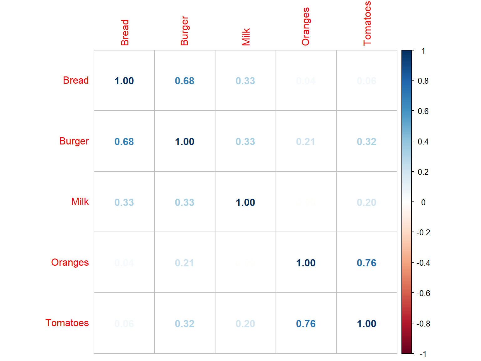
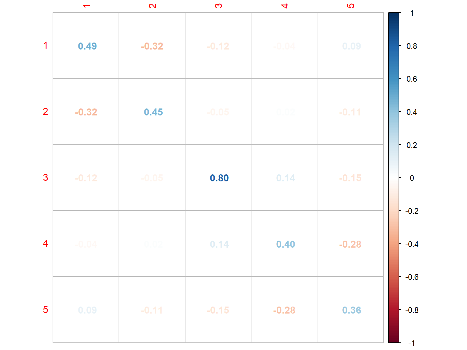
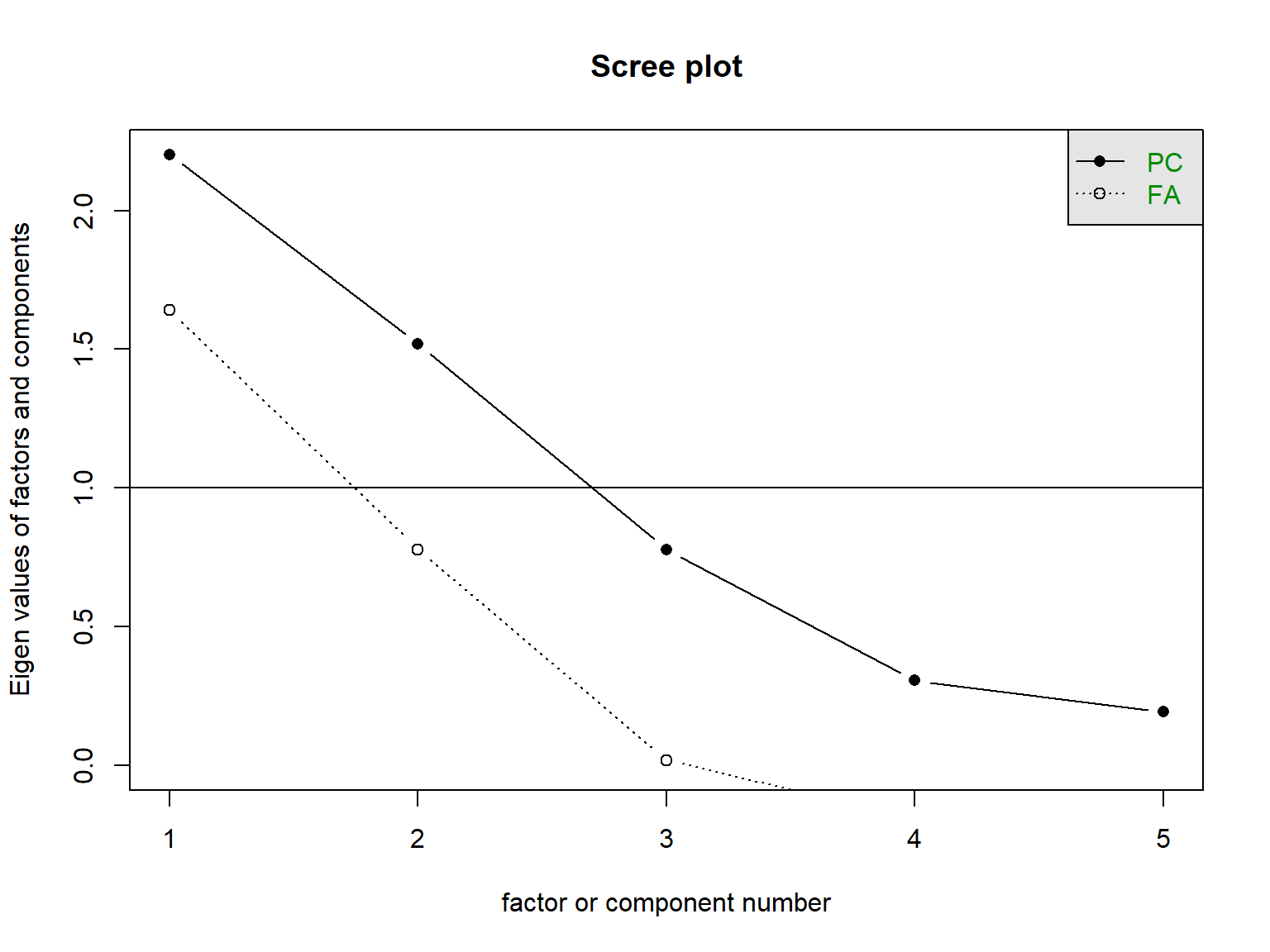
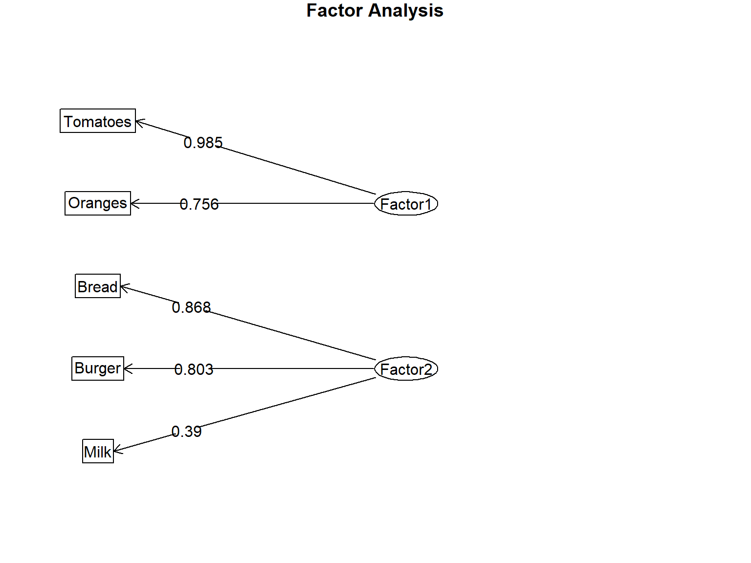
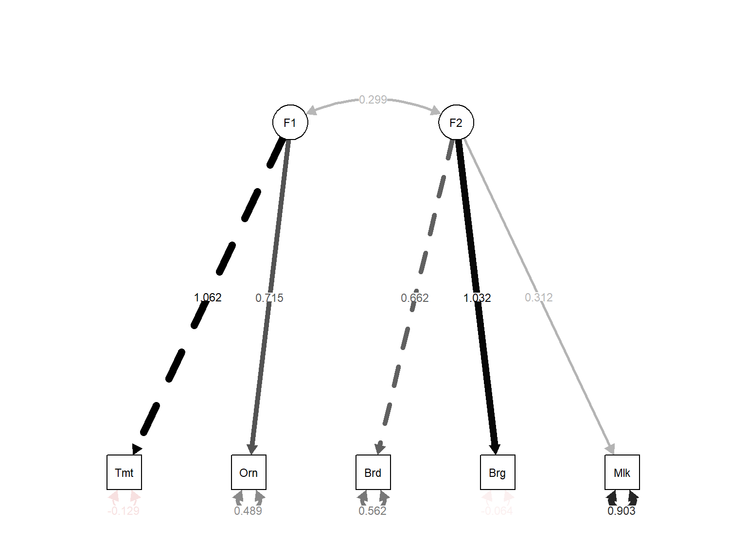
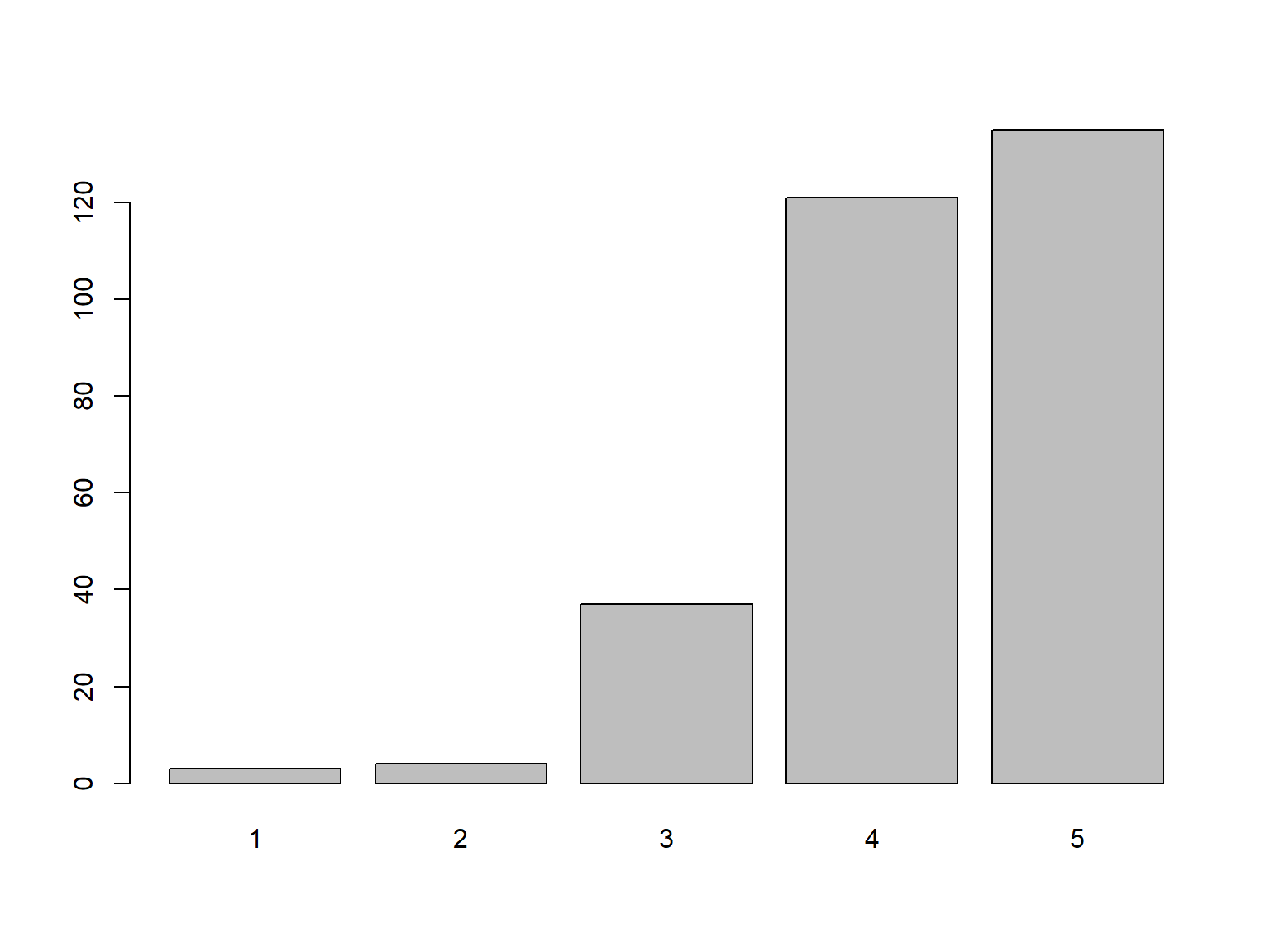
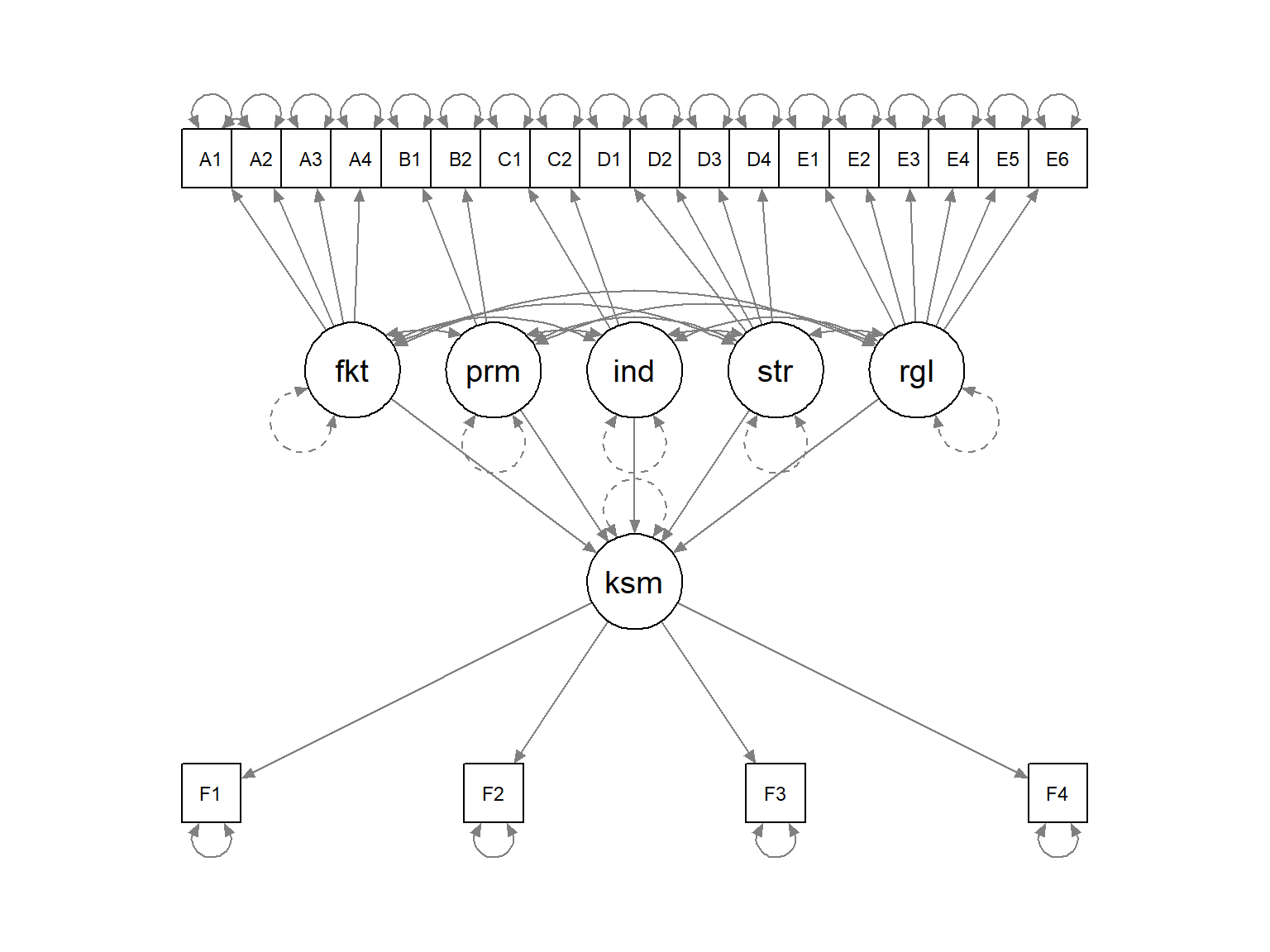
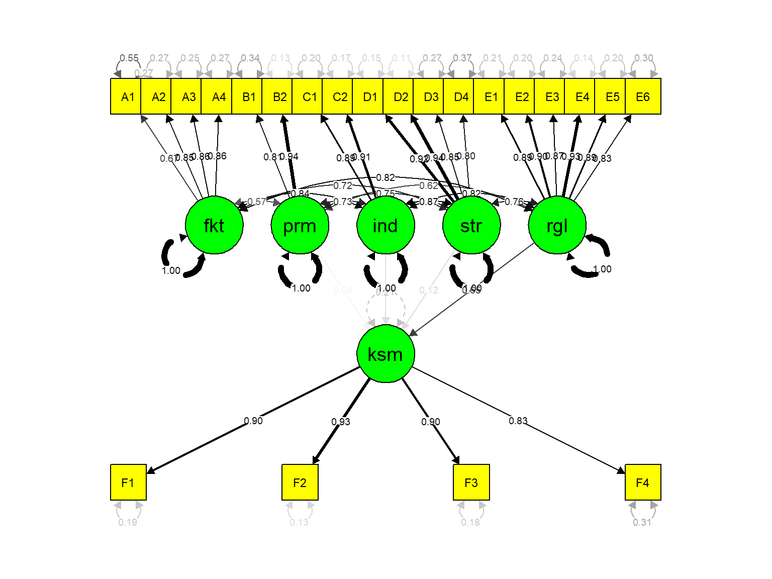
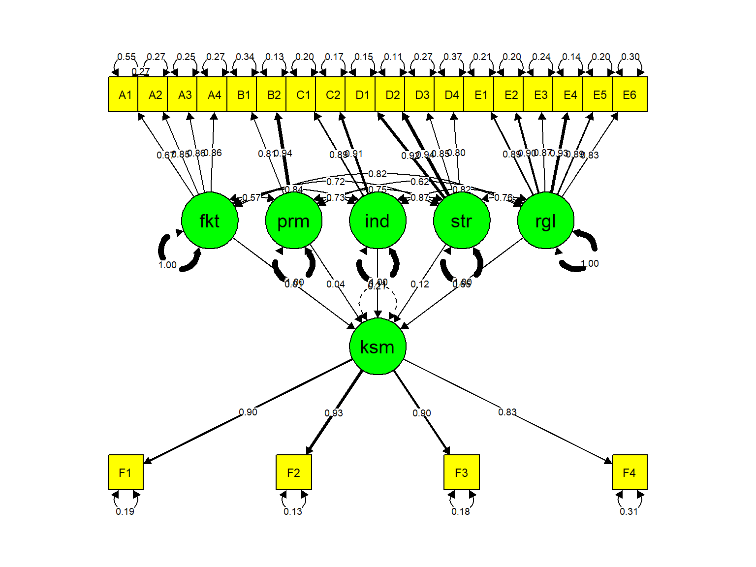
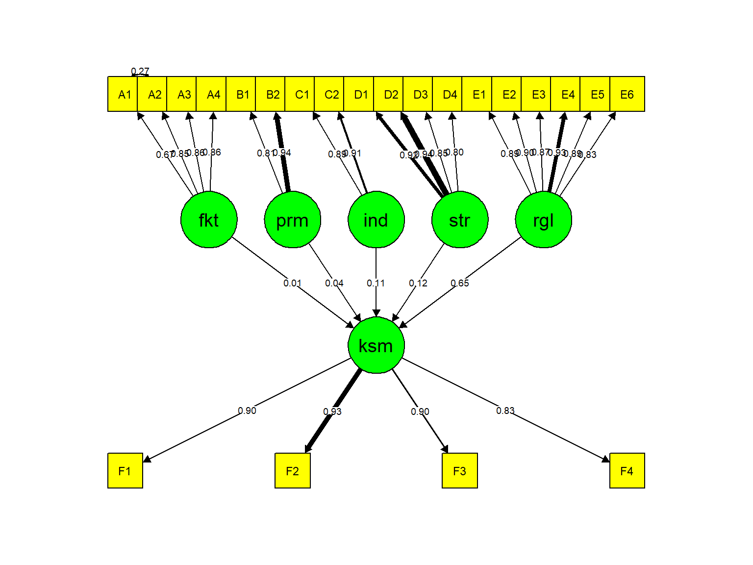
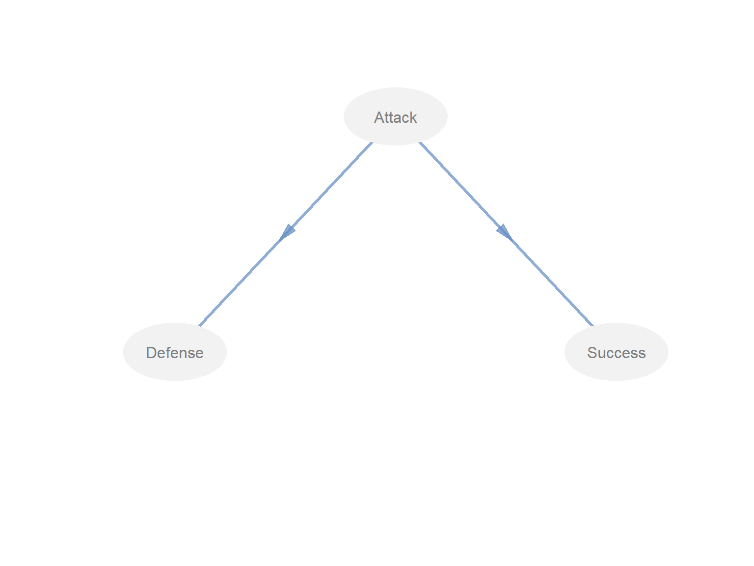
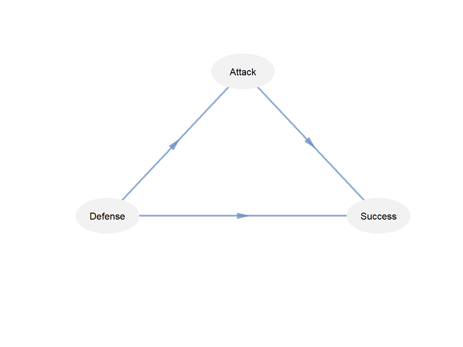
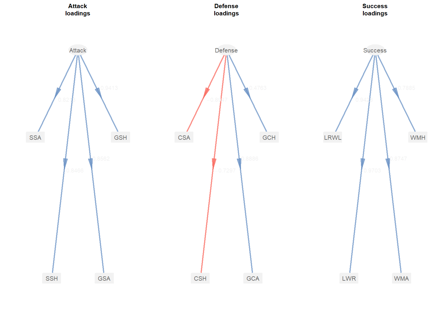
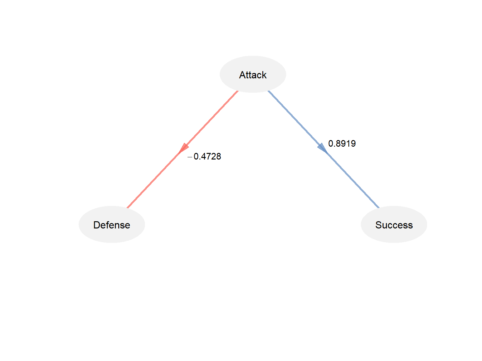
# Factor Analysis and Structural Equation Modeling (SEM) ## Analisis Faktor ```{r} <- read.csv ("Data/harga.csv" )head (harga)``` ```{r} str (harga)``` ### EFA ```{r} library (corrplot)corrplot (cor (harga[,2 : 6 ]), method= "number" )``` ```{r} library (psych)KMO (harga[,2 : 6 ])``` ```{r} # Bartlett's Test of Sphericity cortest.bartlett (harga[,2 : 6 ])``` ```{r} # Anti image correlation (AIC) corrplot (KMO (harga[,2 : 6 ])$ ImCo, method= "number" ) ``` ```{r} # Determinan positif det (cor (harga[,2 : 6 ]))``` ```{r} # Principal component analysis (PCA) = princomp (harga[,2 : 6 ], scores= TRUE , cor= TRUE )summary (pca1)``` ```{r} scree (harga[,2 : 6 ])``` ```{r} # Menentukan faktor loading Analisis faktor loading loadings (pca1)``` ```{r} # Rotasi untuk mengkonfirmasi hasil analisis loading = factanal (harga[,2 : 6 ], factor= 2 , rotation= "varimax" )``` ```{r} # Diagram jalur hasil analisis EFA dan menampilkan faktor loading-nya fa.diagram (fa1$ loadings, digits = 3 )``` ### CFA ```{r} # Spesifikasi model attach (harga)<- " F1 =~ Tomatoes + Oranges F2 =~ Bread + Burger + Milk F1 ~~ F2 " ``` ```{r} library (lavaan)= cfa (model1, data = harga)summary (fitmod, fit.measures = TRUE , standardized = TRUE )``` ```{r} fitmeasures (fitmod)``` ```{r} library (semPlot)semPaths (fitmod, what= 'std' , layout= 'tree' , title = TRUE , posCol = 1 , nDigits = 3 , edge.label.cex= 0.7 , exoVar = FALSE , sizeMan = 5 , sizeLat = 5 )``` ```{r} # Estimasi Reliabilitas alpha cronbach :: alpha (harga[,2 : 6 ])``` ## Model Persamaan Struktural (SEM) ```{r} library (lavaan) library (semPlot)``` ```{r} library (readxl)<- read_excel ("Data/Datalikert.xlsx" )head (datasem[,1 : 5 ])``` ```{r} str (datasem)``` ```{r} attach (datasem)table (A1)``` ```{r} barplot (table (A1))``` ```{r} # Spesifikasi Model = " faktor =~ A1 + A2 + A3 + A4 permintaan =~ B1 + B2 industri =~ C1 + C2 strategi =~ D1 + D2 + D3 + D4 regulasi =~ E1 + E2 + E3 + E4 + E5 + E6 kesempatan =~ F1 + F2 + F3 + F4 kesempatan ~ faktor + permintaan + industri + strategi + regulasi" ``` ```{r} = sem (sem.model, data = datasem)summary (sem.fit, fit.measures= TRUE )``` ```{r} = sem (sem.model, data = datasem, std.lv= TRUE )summary (sem.fit, fit.measures= TRUE , standardized= TRUE )``` ```{r} #sem.fit = sem(sem.model, data = datasem, std.lv=TRUE, orthogonal=TRUE) #summary(sem.fit, fit.measures=TRUE, standardized=TRUE) ``` ```{r} # Modification Indices modificationIndices (sem.fit, minimum.value = 10 )``` ```{r} = " faktor =~ A1 + A2 + A3 + A4 permintaan =~ B1 + B2 industri =~ C1 + C2 strategi =~ D1 + D2 + D3 + D4 regulasi =~ E1 + E2 + E3 + E4 + E5 + E6 kesempatan =~ F1 + F2 + F3 + F4 kesempatan ~ faktor + permintaan + industri + strategi + regulasi A1 ~~ A2 " ``` ```{r} = sem (sem.model2, data = datasem, std.lv= TRUE )summary (sem.fit, fit.measures= TRUE , standardized= TRUE )``` ### Visualisasi SEM ```{r} semPaths (sem.fit)``` ```{r} semPaths (sem.fit, "std" , color = list (lat = "green" , man = "yellow" ), edge.color= "black" )``` ```{r} semPaths (sem.fit, "std" , color = list (lat = "green" , man = "yellow" ), edge.color= "black" , fade= FALSE )``` ```{r} semPaths (sem.fit, "std" , color = list (lat = "green" , man = "yellow" ), edge.color= "black" , fade= FALSE , residuals= FALSE , exoCov= FALSE )``` ## PLS SEM ```{r} # source:https://rpubs.com/ifn1411/PLS # install plspm #install.packages("plspm") # load plspm library (plspm)``` ```{r} # load data spainmodel data (spainfoot)# first 5 row of spainmodel data head (spainfoot)``` ```{r} <- c (0 , 0 , 0 )<- c (1 , 0 , 0 )<- c (1 , 0 , 0 )<- rbind (Attack, Defense, Success)colnames (model_path) <- rownames (model_path)``` ```{r} # graph structural model innerplot (model_path)``` ```{r} <- c (0 , 1 , 0 )<- c (0 , 0 , 0 )<- c (1 , 1 , 0 )<- rbind (Attack, Defense, Success)colnames (model_path2) <- rownames (model_path2)``` ```{r} # graph structural model innerplot (model_path2, txt.col = "black" )``` ```{r} # define latent variable associated with <- list (1 : 4 , 5 : 8 , 9 : 12 )# vector of modes (reflective) <- c ("A" , "A" , "A" )# run plspm analysis <- plspm (Data = spainfoot, path_matrix = model_path, blocks = model_blocks, modes = model_modes)``` ```{r} # Unidimensionality $ unidim``` ```{r} plot (model_pls, what = "loadings" )``` ```{r} # Loadings and Communilaties $ outer_model``` ```{r} # Crossloadings $ crossloadings``` ```{r} # Coefficient of Determination $ inner_model``` ```{r} # Redundancy $ inner_summary``` ```{r} # Goodness-of-fit $ gof``` ```{r} plot (model_pls, what = "inner" , colpos = "#6890c4BB" , colneg = "#f9675dBB" , txt.col = "black" , arr.tcol= "black" )```