Metode berhirarki
Ref: https://rpubs.com/odenipinedo/cluster-analysis-in-R
library(readxl)
Provinsi <- read_excel("Data/provinsi.xlsx")
Prov.scaled = scale(Provinsi[,c(4:8)])
rownames(Prov.scaled) = Provinsi$Provinsi
head(Prov.scaled)
               IPM         UHH        RLS         PPK       Gini
Aceh    0.20822137  0.04044611  0.7444782 -0.62264434 -0.8089350
Sumut   0.20085709 -0.39282591  1.0245728 -0.11277090 -0.6516207
Sumbar  0.36532598 -0.23835502  0.4747574  0.01481560 -1.2546590
Riau    0.50033775  0.59428078  0.5162529  0.19012890 -0.9138112
Jambi   0.05848104  0.50762638 -0.1165536 -0.18648754 -0.6778397
Sumsel -0.21890679 -0.08765171 -0.2825356 -0.02582306  0.1349510
## membuat dissimilarity matrix
dprov = dist(Prov.scaled, method="euclidean")
c.comp = hclust(dprov, method = "complete")
cor(dprov , cophenetic(c.comp))
c.sing = hclust(dprov, method = "single")
cor(dprov , cophenetic(c.sing))
c.avrg = hclust(dprov, method = "average")
cor(dprov , cophenetic(c.avrg))
c.ward = hclust(dprov, method = "ward.D")
cor(dprov , cophenetic(c.ward))
c.ctrd = hclust(dprov, method = "centroid")
cor(dprov , cophenetic(c.ctrd))
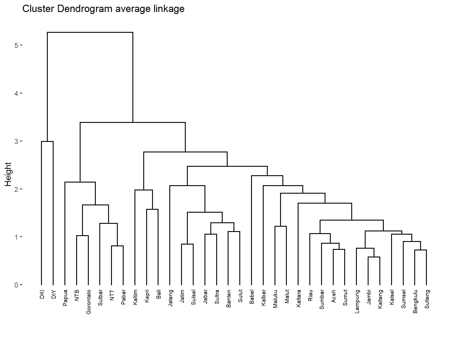
library(factoextra)
fviz_dend(c.avrg, cex = 0.5,
          main = "Cluster Dendrogram average linkage")
avg_coph <- cophenetic(c.avrg)
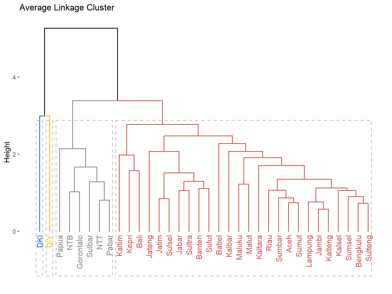
avg_clust <- cutree(c.avrg, k = 4)
table(avg_clust)
avg_clust
 1  2  3  4
26  1  1  6
fviz_dend(c.avrg, k = 4,
          k_colors = "jco",
          rect = T,
          main = "Average Linkage Cluster")
library(clValid)
library(cluster)
# internal measures
internal <- clValid(Prov.scaled, nClust = 2:6,
                    clMethods = "hierarchical",
                    validation = "internal",
                    metric = "euclidean",
                    method = "average")
summary(internal)
Clustering Methods:
 hierarchical

Cluster sizes:
 2 3 4 5 6

Validation Measures:
                                 2       3       4       5       6

hierarchical Connectivity   4.5246 10.3012 11.6345 18.3198 24.1508
             Dunn           0.3637  0.3703  0.3703  0.3224  0.3592
             Silhouette     0.4915  0.3484  0.3092  0.2567  0.3117

Optimal Scores:

             Score  Method       Clusters
Connectivity 4.5246 hierarchical 2
Dunn         0.3703 hierarchical 3
Silhouette   0.4915 hierarchical 2
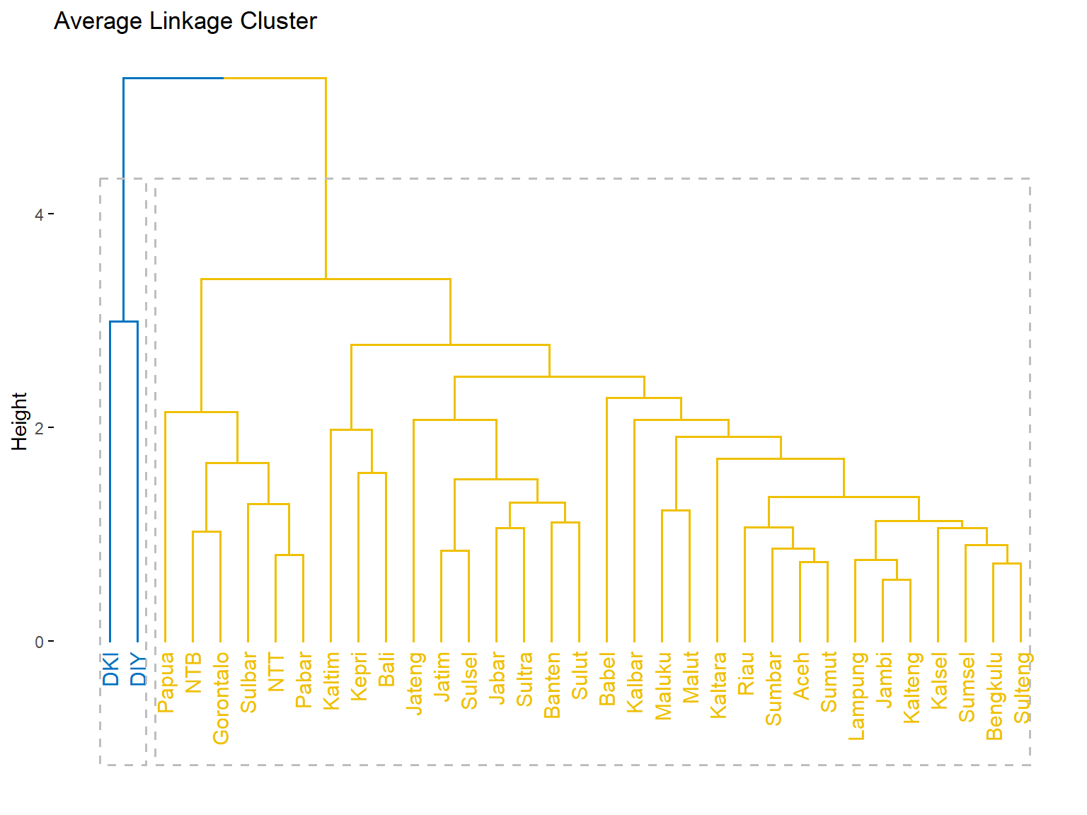
fviz_dend(c.avrg, k = 2,
          k_colors = "jco",
          rect = T,
          main = "Average Linkage Cluster")
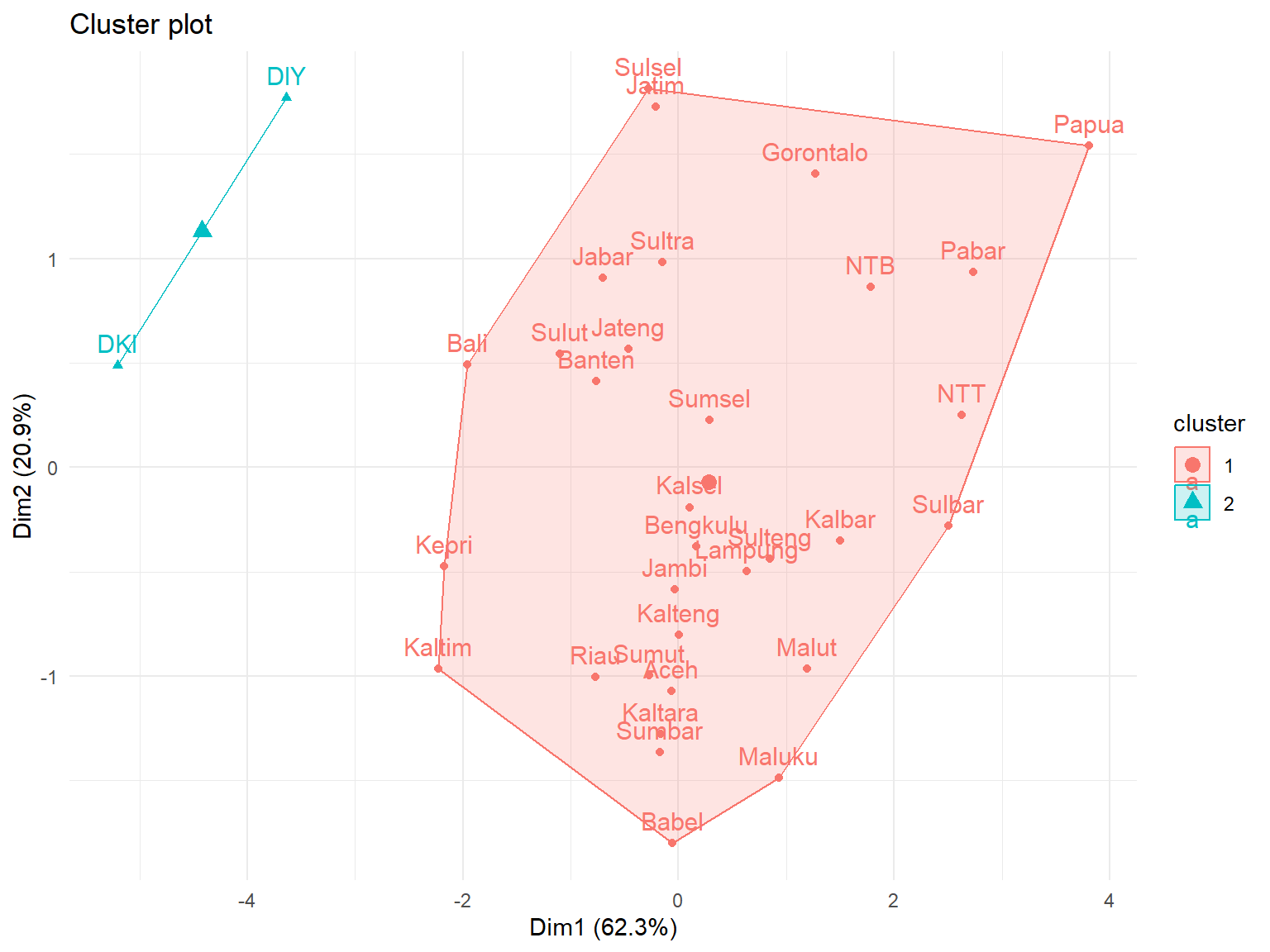
group = cutree(c.avrg, k = 2)
group
     Aceh     Sumut    Sumbar      Riau     Jambi    Sumsel  Bengkulu   Lampung
        1         1         1         1         1         1         1         1
    Babel     Kepri       DKI     Jabar    Jateng       DIY     Jatim    Banten
        1         1         2         1         1         2         1         1
     Bali       NTB       NTT    Kalbar   Kalteng    Kalsel    Kaltim   Kaltara
        1         1         1         1         1         1         1         1
    Sulut   Sulteng    Sulsel    Sultra Gorontalo    Sulbar    Maluku     Malut
        1         1         1         1         1         1         1         1
    Pabar     Papua
        1         1
fviz_cluster(list(data = Prov.scaled,
                  cluster = group)) +
  theme_minimal()
Standard deviations (1, .., p=5):
[1] 1.7653705 1.0227284 0.7270850 0.5299864 0.1671984

Rotation (n x k) = (5 x 5):
            PC1         PC2          PC3           PC4         PC5
IPM  -0.5601680 -0.05311199 -0.005227509 -0.0006949187 -0.82665781
UHH  -0.4513030  0.05646383 -0.811065327  0.2024129889  0.30714735
RLS  -0.4591728 -0.33781331  0.497619343  0.5648220282  0.32923179
PPK  -0.5069166  0.09086739  0.227624805 -0.7546468667  0.33685862
Gini -0.1213811  0.93360390  0.206658283  0.2655422416  0.02073819
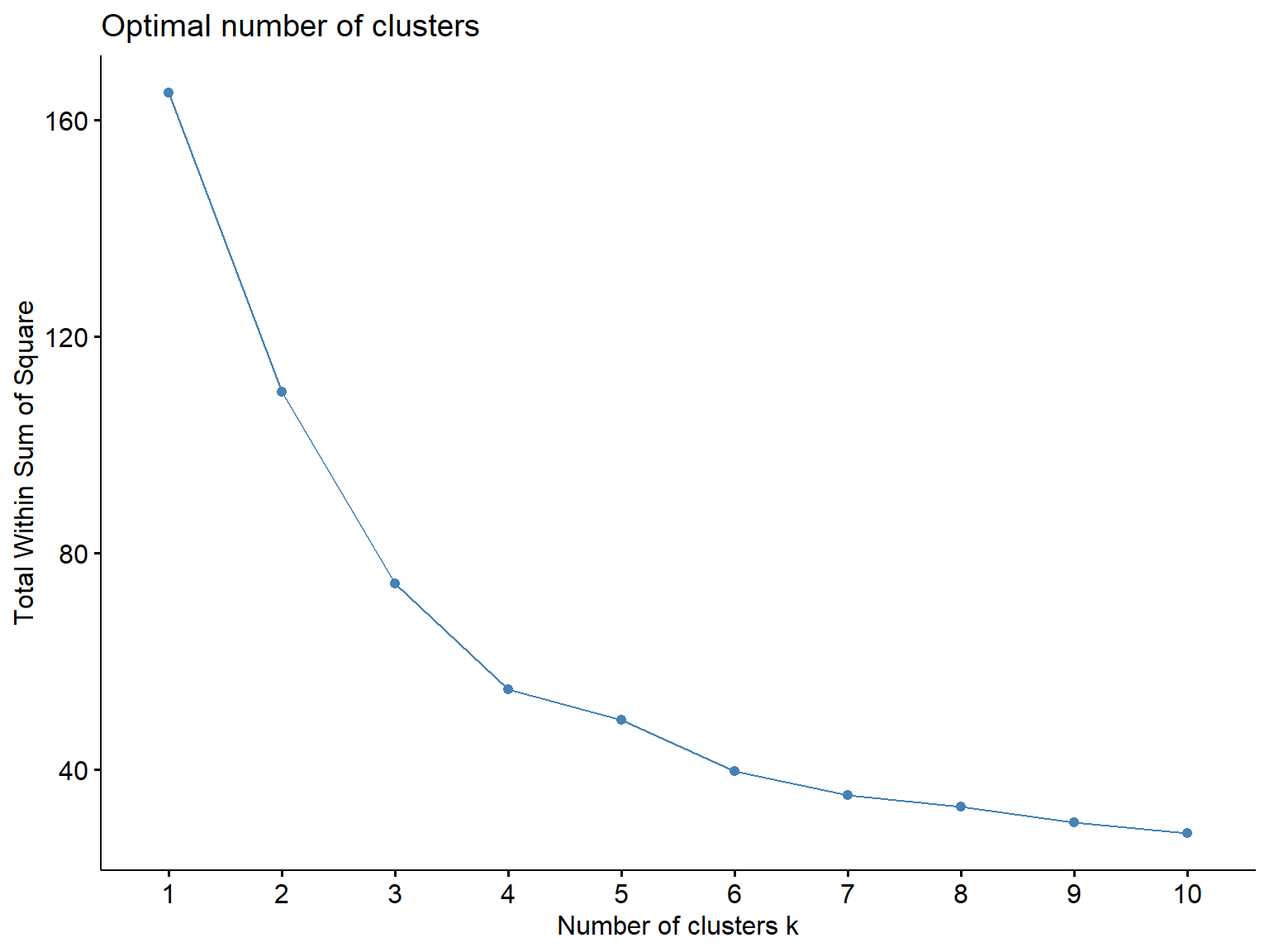
Metode tidak berhirarki - kmeans
fviz_nbclust(Prov.scaled, kmeans, method = "wss")
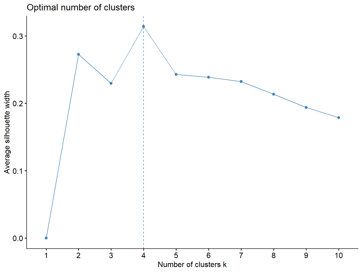
fviz_nbclust(Prov.scaled, kmeans, method = "silhouette")
set.seed(1)
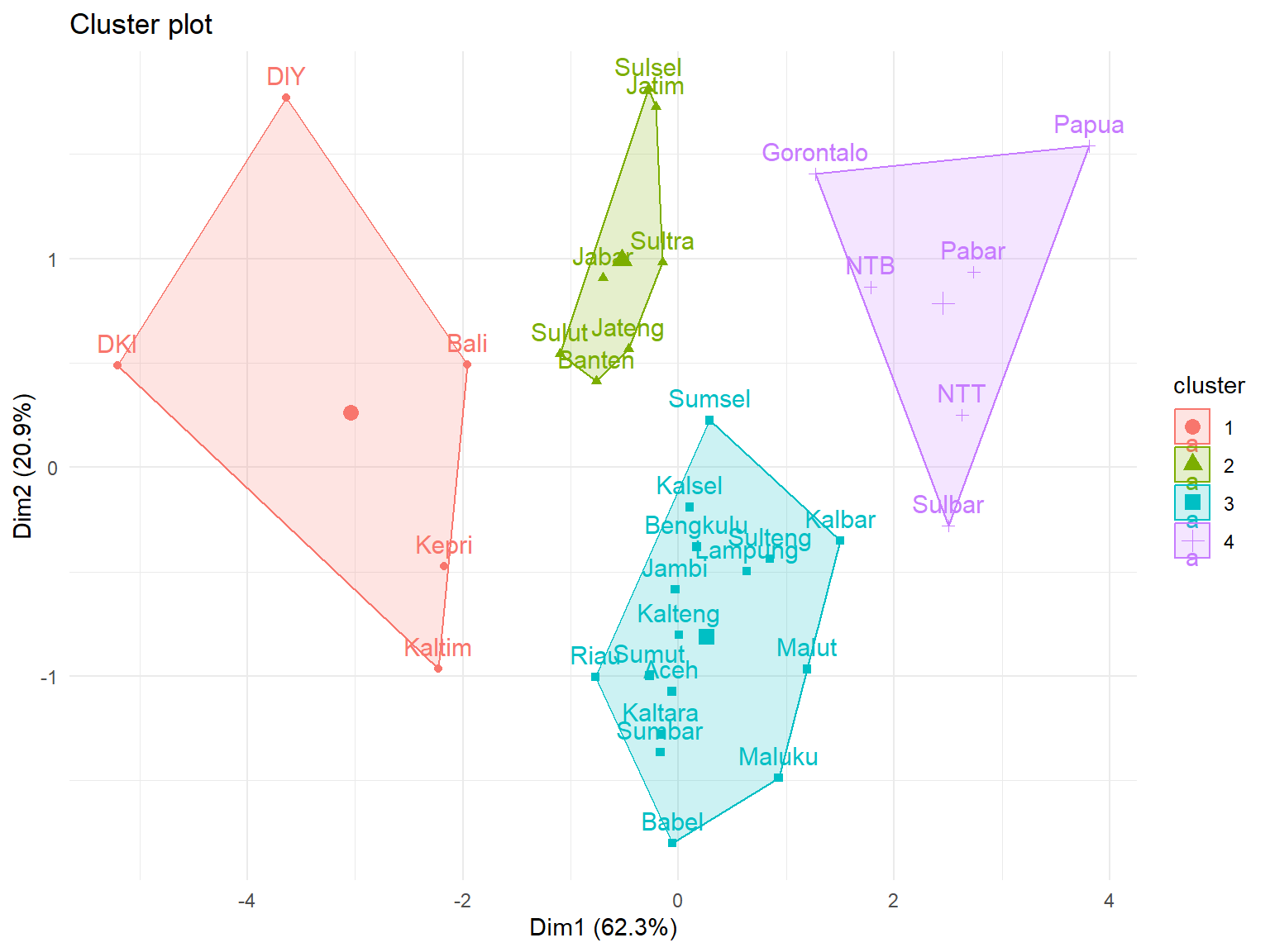
km = kmeans(Prov.scaled, centers=4)
km
K-means clustering with 4 clusters of sizes 5, 7, 16, 6

Cluster means:
          IPM        UHH        RLS         PPK       Gini
1  1.67223995  1.1202353  1.3689855  1.75840321  0.6331131
2  0.22785944  0.6620973 -0.1491572  0.09292014  0.9739608
3 -0.08819085 -0.1001318  0.1246391 -0.24567350 -0.7991029
4 -1.42419372 -1.4389581 -1.2991755 -0.91861351  0.4670591

Clustering vector:
     Aceh     Sumut    Sumbar      Riau     Jambi    Sumsel  Bengkulu   Lampung
        3         3         3         3         3         3         3         3
    Babel     Kepri       DKI     Jabar    Jateng       DIY     Jatim    Banten
        3         1         1         2         2         1         2         2
     Bali       NTB       NTT    Kalbar   Kalteng    Kalsel    Kaltim   Kaltara
        1         4         4         3         3         3         1         3
    Sulut   Sulteng    Sulsel    Sultra Gorontalo    Sulbar    Maluku     Malut
        2         3         2         2         4         4         3         3
    Pabar     Papua
        4         4

Within cluster sum of squares by cluster:
[1] 17.054859  7.933134 22.111511  7.711994
 (between_SS / total_SS =  66.8 %)

Available components:

[1] "cluster"      "centers"      "totss"        "withinss"     "tot.withinss"
[6] "betweenss"    "size"         "iter"         "ifault"
fviz_cluster(list(data = Prov.scaled, cluster = km$cluster)) + theme_minimal()