Latihan Pasca-Workshop

Latihan opsional untuk menguji pengetahuan dan memperkuat pemahaman Anda

Persiapan

Siapkan cheatsheet dplyr, tidyr, dan ggplot agar mudah dirujuk.

Muat paket-paket

Kode di bawah ini akan memuat paket-paket yang Anda butuhkan:

library(tidyverse)
library(car)

Muat dataset

Kode di bawah ini akan memuat dan menampilkan beberapa baris pertama dari dataset Duncan. Untuk mengetahui lebih lanjut tentang dataset ini, ketik ?Duncan di konsol RStudio Anda.

duncan <- as_tibble(Duncan)
print(duncan)

# A tibble: 45 × 4
   type  income education prestige
   <fct>  <int>     <int>    <int>
 1 prof      62        86       82
 2 prof      72        76       83
 3 prof      75        92       90
 4 prof      55        90       76
 5 prof      64        86       90
 6 prof      21        84       87
 7 prof      64        93       93
 8 prof      80       100       90
 9 wc        67        87       52
10 prof      72        86       88
# ℹ 35 more rows

Kode di bawah ini akan memuat dan menampilkan beberapa baris pertama dari dataset WVS. Untuk mengetahui lebih lanjut tentang dataset ini, ketik ?WVS di konsol RStudio Anda.

wvs <- as_tibble(WVS)
print(wvs)

# A tibble: 5,381 × 6
   poverty     religion degree country   age gender
   <ord>       <fct>    <fct>  <fct>   <int> <fct> 
 1 Too Little  yes      no     USA        44 male  
 2 About Right yes      no     USA        40 female
 3 Too Little  yes      no     USA        36 female
 4 Too Much    yes      yes    USA        25 female
 5 Too Little  yes      yes    USA        39 male  
 6 About Right yes      no     USA        80 female
 7 Too Much    yes      no     USA        48 female
 8 Too Little  yes      no     USA        32 male  
 9 Too Little  yes      no     USA        74 female
10 Too Little  yes      no     USA        30 male  
# ℹ 5,371 more rows

Soal 1

Menggunakan dataset wvs, filter kolom age untuk menyertakan nilai lebih dari 29. Kemudian, pilih kolom age, degree, religion dan poverty. Simpan hasilnya ke dataframe baru bernama wvs_filtered.

Show Answer

wvs_filtered <- wvs |> 
    filter(age > 29) |> 
    select(age, degree, religion, poverty) 

print(wvs_filtered)

# A tibble: 4,228 × 4
     age degree religion poverty    
   <int> <fct>  <fct>    <ord>      
 1    44 no     yes      Too Little 
 2    40 no     yes      About Right
 3    36 no     yes      Too Little 
 4    39 yes    yes      Too Little 
 5    80 no     yes      About Right
 6    48 no     yes      Too Much   
 7    32 no     yes      Too Little 
 8    74 no     yes      Too Little 
 9    30 no     yes      Too Little 
10    32 yes    yes      Too Little 
# ℹ 4,218 more rows

Soal 2

Perbarui dataset wvs dengan membuat versi dummy-coded dari variabel gender, di mana male = 0 dan female = 1. Simpan hasilnya di kolom baru bernama gender_coded.

Show Answer

wvs <- wvs |> 
    mutate(gender_coded = if_else(gender == "male", 0, 1)) 

print(wvs)

# A tibble: 5,381 × 7
   poverty     religion degree country   age gender gender_coded
   <ord>       <fct>    <fct>  <fct>   <int> <fct>         <dbl>
 1 Too Little  yes      no     USA        44 male              0
 2 About Right yes      no     USA        40 female            1
 3 Too Little  yes      no     USA        36 female            1
 4 Too Much    yes      yes    USA        25 female            1
 5 Too Little  yes      yes    USA        39 male              0
 6 About Right yes      no     USA        80 female            1
 7 Too Much    yes      no     USA        48 female            1
 8 Too Little  yes      no     USA        32 male              0
 9 Too Little  yes      no     USA        74 female            1
10 Too Little  yes      no     USA        30 male              0
# ℹ 5,371 more rows

Soal 3

Buat ringkasan dari dataset wvs yang menampilkan jumlah observasi untuk setiap negara.

Show Answer

wvs |> 
    count(country)

# A tibble: 4 × 2
  country       n
  <fct>     <int>
1 Australia  1874
2 Norway     1127
3 Sweden     1003
4 USA        1377

Soal 4

Menggunakan dataset wvs, hitung rata-rata age untuk setiap kombinasi gender dan status gelar.

Show Answer

wvs |> 
    group_by(gender, degree) |> 
    summarise(avg_age = mean(age, na.rm = TRUE))

`summarise()` has grouped output by 'gender'. You can override using the
`.groups` argument.

# A tibble: 4 × 3
# Groups:   gender [2]
  gender degree avg_age
  <fct>  <fct>    <dbl>
1 female no        45.6
2 female yes       41.0
3 male   no        46.0
4 male   yes       43.3

Soal 5

Menggunakan dataset wvs, buat statistik ringkasan untuk setiap negara dan agama (yes/no). Hitung age mean, age median, dan jumlah observasi.

Show Answer

wvs |> 
    group_by(country, religion) %>%
    summarise(
        avg_age = mean(age, na.rm = TRUE),
        median_age = median(age, na.rm = TRUE),
        n_observations = n()
    )

`summarise()` has grouped output by 'country'. You can override using the
`.groups` argument.

# A tibble: 8 × 5
# Groups:   country [4]
  country   religion avg_age median_age n_observations
  <fct>     <fct>      <dbl>      <dbl>          <int>
1 Australia no          39.9         37            375
2 Australia yes         45.7         43           1499
3 Norway    no          40.6         38            109
4 Norway    yes         43.6         42           1018
5 Sweden    no          43.7         42             15
6 Sweden    yes         43.9         43            988
7 USA       no          44.6         42            287
8 USA       yes         48.9         46           1090

Soal 6

Menggunakan dataset wvs, pilih 10 responden tertua dari USA. (petunjuk: arrange() dan slice())

Show Answer

wvs |> 
    filter(country == "USA", age > 50) |> 
    arrange(desc(age)) |> 
    slice(1:10)

# A tibble: 10 × 7
   poverty     religion degree country   age gender gender_coded
   <ord>       <fct>    <fct>  <fct>   <int> <fct>         <dbl>
 1 Too Much    no       no     USA        91 male              0
 2 Too Little  yes      no     USA        91 male              0
 3 Too Much    yes      no     USA        88 female            1
 4 About Right yes      no     USA        88 male              0
 5 Too Little  yes      yes    USA        87 female            1
 6 Too Much    yes      no     USA        87 female            1
 7 Too Little  yes      no     USA        87 male              0
 8 About Right yes      no     USA        87 male              0
 9 About Right yes      no     USA        86 female            1
10 Too Much    yes      no     USA        86 female            1

Soal 7

Perbarui dataset wvs dengan menambahkan kolom baru bernama age_category yang mengkategorikan setiap responden berdasarkan kriteria berikut:

below 18 = “youth” category
between 18 to 34 = “young adult” category
between 35 to 49 = “adult” category
between 50 to 69 = “senior” category
more than 70 = “elderly” category

Show Answer

wvs <- wvs |> 
    mutate(age_category = case_when(
        age < 18 ~ "youth",
        age >= 18 & age < 35 ~ "young adult",
        age >= 35 & age < 50 ~ "adult",
        age >= 50 & age < 70 ~ "senior",
        age >= 70 ~ "elderly"
    )) 

print(wvs)

# A tibble: 5,381 × 8
   poverty     religion degree country   age gender gender_coded age_category
   <ord>       <fct>    <fct>  <fct>   <int> <fct>         <dbl> <chr>       
 1 Too Little  yes      no     USA        44 male              0 adult       
 2 About Right yes      no     USA        40 female            1 adult       
 3 Too Little  yes      no     USA        36 female            1 adult       
 4 Too Much    yes      yes    USA        25 female            1 young adult 
 5 Too Little  yes      yes    USA        39 male              0 adult       
 6 About Right yes      no     USA        80 female            1 elderly     
 7 Too Much    yes      no     USA        48 female            1 adult       
 8 Too Little  yes      no     USA        32 male              0 young adult 
 9 Too Little  yes      no     USA        74 female            1 elderly     
10 Too Little  yes      no     USA        30 male              0 young adult 
# ℹ 5,371 more rows

Soal 8

Buat ulang visualisasi berikut:

Show Answer

wvs |> ggplot(aes(x = country, fill = poverty)) +
    geom_bar(position = "dodge") +
    labs(title = "Distribution of Poverty Opinions Across Countries",
       x = "Country", 
       y = "Count", 
       fill = "Poverty Opinion") +
    theme_minimal()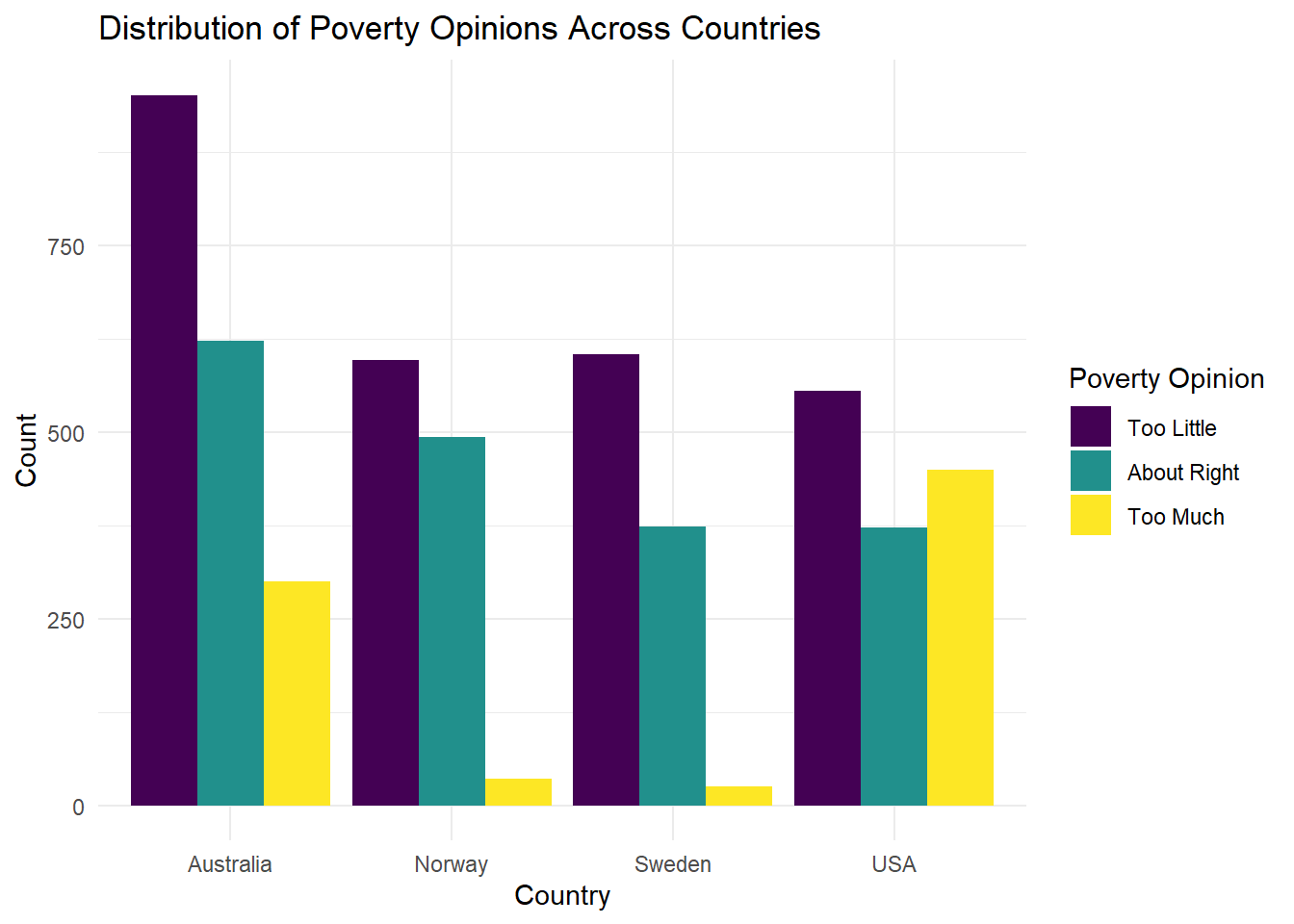

Soal 9

Buat ulang visualisasi berikut:

Show Answer

wvs |> 
    ggplot(aes(x = country, fill = degree)) +
    geom_bar(position = "fill") +
    labs(title = "Proportion of Degree Status by Country", 
       x = "Country", y = "Count", fill = "Degree Status") +
    theme_minimal()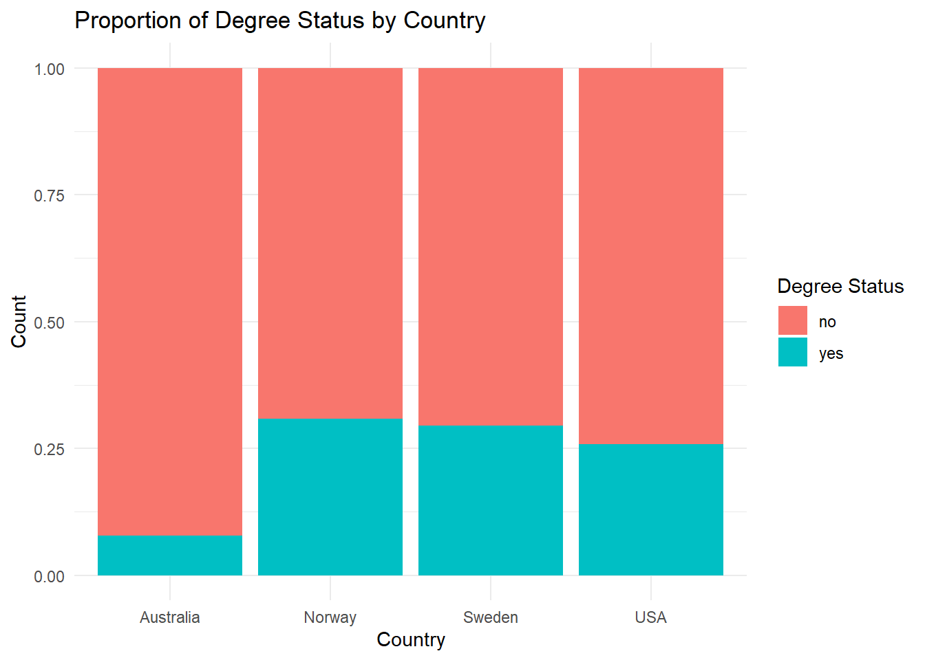

Soal 10

Buat ulang visualisasi berikut:

Show Answer

wvs |> ggplot(aes(x = country, y = age)) +
    geom_boxplot() +
    labs(title = "Age Distribution by Country", x = "Country", y = "Age") +
    theme_minimal() +
    theme(legend.position = "none")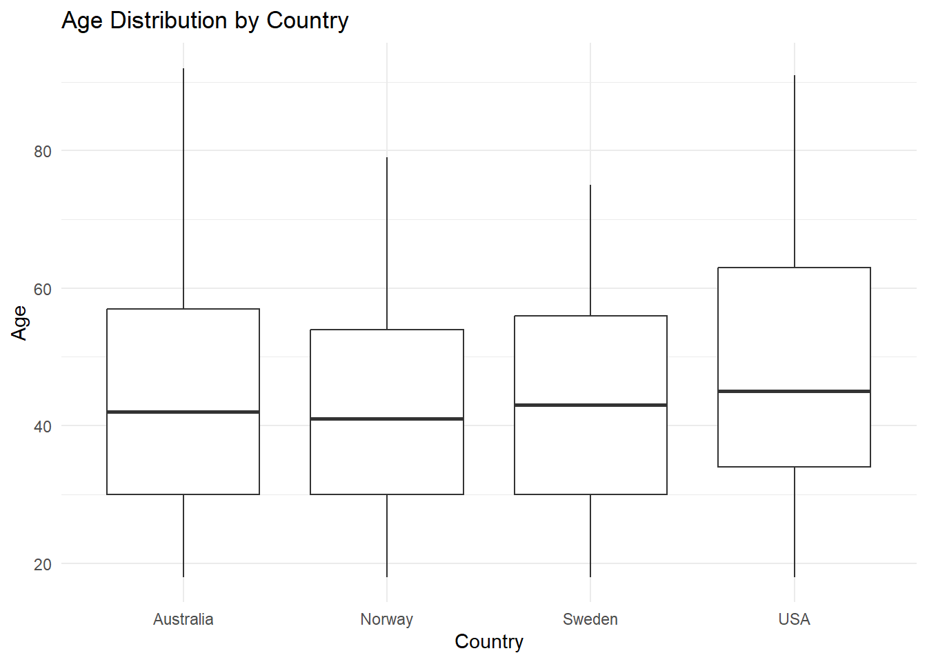

Soal 11

Buat ulang visualisasi berikut:

Show Answer

wvs |> 
    ggplot(aes(x = country, y = age)) +
    geom_boxplot() +
    facet_wrap(~ religion) +
    labs(title = "Age Distribution by Country and Religion",
       x = "Country", y = "Age") +
    theme_minimal()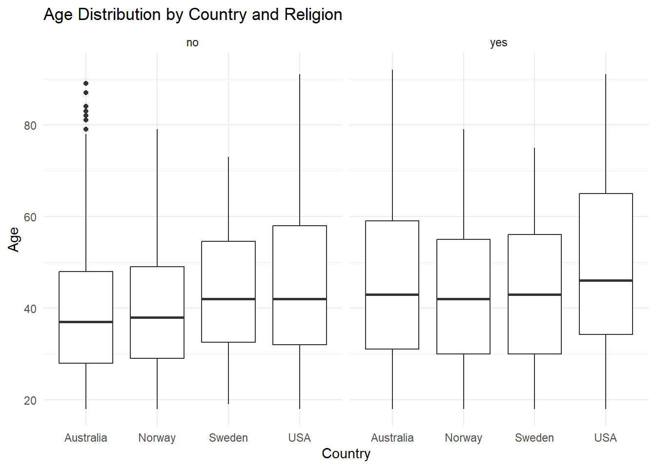

Soal 12

Buat ulang visualisasi berikut menggunakan dataset duncan:

Show Answer

duncan |> 
    ggplot(aes(x = income, y = prestige, color = type)) +
    geom_jitter() +
    labs(title = "Occupation Prestige vs. Income",
       x = "Income", 
       y = "Prestige Score",
       color = "Occupation Type") +
    theme_minimal()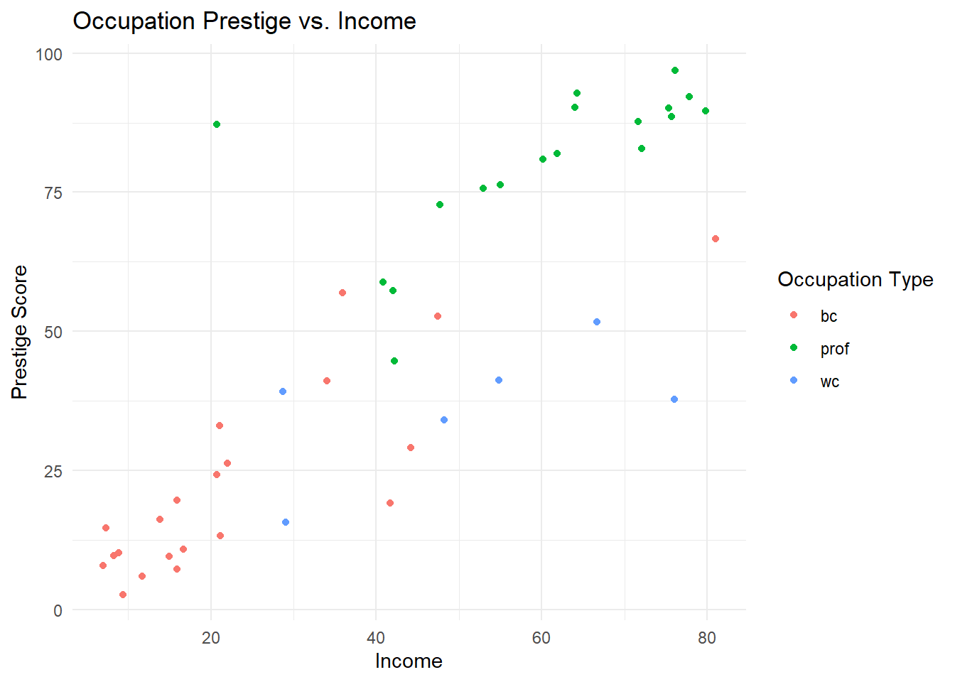

Soal 13

Buat ulang visualisasi berikut menggunakan dataset duncan:

Show Answer

duncan |> 
    ggplot(aes(x = type, y = income)) +
    geom_boxplot() +
    labs(title = "Income Distribution by Occupation Type",
        x = "Occupation Type",
        y = "Income") +
    theme_minimal()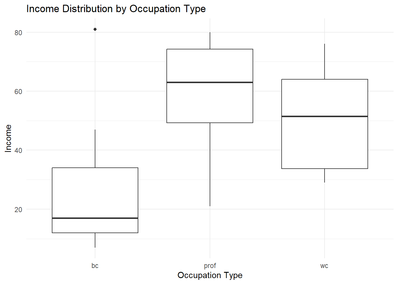

Soal 14

Buat ulang visualisasi berikut menggunakan dataset duncan:

Show Answer

duncan |> 
    ggplot(aes(x = prestige, y = income, color = type)) +
    geom_jitter() +
    geom_smooth(method = "lm") +
    labs(
        title = "Relationship between Prestige and Income",
        subtitle = "Grouped by Occupation Type",
        x = "Prestige Score",
        y = "Income",
        color = "Occupation Type"
    ) + 
    theme_minimal()

`geom_smooth()` using formula = 'y ~ x'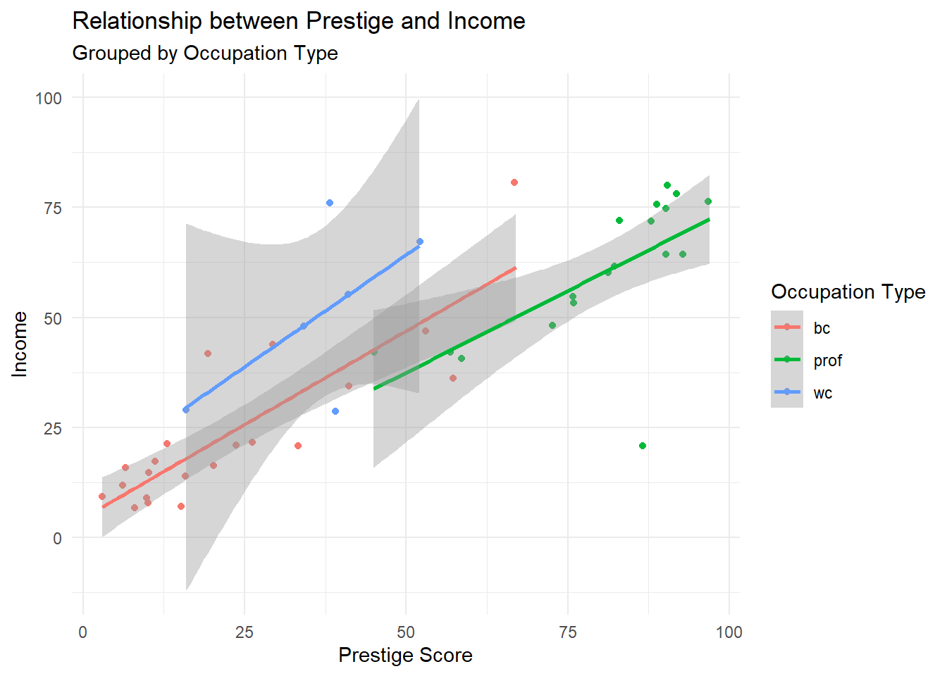

Soal 15

Menggunakan dataset duncan:

Periksa korelasi antara skor prestige dan education.
Analisis hubungan antara income dan skor prestige.

Show Answer

cor.test(duncan$prestige, duncan$education)


    Pearson's product-moment correlation

data:  duncan$prestige and duncan$education
t = 10.668, df = 43, p-value = 1.171e-13
alternative hypothesis: true correlation is not equal to 0
95 percent confidence interval:
 0.7445746 0.9163112
sample estimates:
      cor 
0.8519156

Show Answer

cor.test(duncan$prestige, duncan$income)


    Pearson's product-moment correlation

data:  duncan$prestige and duncan$income
t = 10.062, df = 43, p-value = 7.144e-13
alternative hypothesis: true correlation is not equal to 0
95 percent confidence interval:
 0.7217665 0.9080298
sample estimates:
      cor 
0.8378014

Soal 16

Menggunakan dataset duncan, bandingkan skor prestige antar kategori pekerjaan yang berbeda menggunakan ANOVA.

Show Answer

duncan_anova <- aov(prestige ~ type, data=duncan)
summary(duncan_anova)

            Df Sum Sq Mean Sq F value   Pr(>F)    
type         2  33090   16545   65.57 1.21e-13 ***
Residuals   42  10598     252                     
---
Signif. codes:  0 '***' 0.001 '**' 0.01 '*' 0.05 '.' 0.1 ' ' 1

Soal 17

Menggunakan dataset duncan, buat model regresi yang memprediksi income berdasarkan skor prestige dan education.

library(huxtable)

Show Answer

duncan_model <- lm(income ~ prestige + education, data = duncan)
huxreg("income" = duncan_model)

	income
(Intercept)	10.426 *
	(4.164)
prestige	0.624 ***
	(0.125)
education	0.032
	(0.132)
N	45
R2	0.702
logLik	-179.902
AIC	367.805
* p < 0.001; p < 0.01; * p < 0.05.

Soal 18

Menggunakan dataset wvs, periksa hubungan antara religion dan persepsi poverty.

Show Answer

wvs_chisq <- chisq.test(table(wvs$religion, wvs$poverty))
print(wvs_chisq)


    Pearson's Chi-squared test

data:  table(wvs$religion, wvs$poverty)
X-squared = 0.083005, df = 2, p-value = 0.9593

Soal 19

Menggunakan dataset wvs, periksa apakah ada perbedaan signifikan dalam rata-rata usia antara individu dengan dan tanpa gelar universitas.

Show Answer

wvs_ttest <- t.test(age ~ degree, data = wvs)
print(wvs_ttest)


    Welch Two Sample t-test

data:  age by degree
t = 7.0571, df = 2029, p-value = 2.325e-12
alternative hypothesis: true difference in means between group no and group yes is not equal to 0
95 percent confidence interval:
 2.674321 4.732708
sample estimates:
 mean in group no mean in group yes 
         45.82775          42.12423

Soal 20

Menggunakan dataset wvs, bandingkan rata-rata usia antar negara dan kategori usia yang berbeda (lihat Soal 7 untuk membuat age_category), dan selidiki apakah ada perbedaan signifikan. Lakukan uji post-hoc jika diperlukan.

Show Answer

wvs_anova <- aov(age ~ country + age_category, data = wvs)
summary(wvs_anova)

               Df  Sum Sq Mean Sq F value Pr(>F)    
country         3   17399    5800   235.9 <2e-16 ***
age_category    3 1424858  474953 19319.9 <2e-16 ***
Residuals    5374  132113      25                   
---
Signif. codes:  0 '***' 0.001 '**' 0.01 '*' 0.05 '.' 0.1 ' ' 1