Structural Equation Modelling (SEM)

ISEI Workshop

Rencana Hari Ini

Bagian A: CB-SEM dengan lavaan

Two-Step Approach: CFA → Full SEM
Fit indices, reliabilitas, validitas, mediasi

Bagian B: PLS-SEM dengan seminr

Berbagai tipe konstruk (composite, reflective, HOC, formatif)
Outer & inner model evaluation, bootstrap, mediasi

Apa itu SEM?

SEM = analisis faktor + regresi. Menguji hubungan simultan antara variabel laten melalui indikator terukur.

Measurement model: hubungan laten ↔︎ indikator
Structural model: hubungan antar laten

Terminologi SEM

Istilah	Penjelasan
Variabel Laten	Konstruk tidak langsung terukur (oval)
Variabel Manifes	Item kuesioner (kotak)
Variabel Eksogen	Independen — tidak diprediksi variabel lain
Variabel Endogen	Dependen — diprediksi variabel lain

CB-SEM vs PLS-SEM

Kriteria	CB-SEM	PLS-SEM
Basis	Kovarians	Varians
Tujuan	Konfirmasi teori	Prediksi & eksplorasi
Ukuran sampel	Besar (>200)	Kecil–menengah (>50)
Tipe indikator	Reflektif	Reflektif & formatif
Fit indices	CFI, TLI, RMSEA, SRMR	R², HTMT
Paket R	`lavaan`	`seminr`

Two-Step Approach

Anderson & Gerbing (1988):

CFA: Evaluasi measurement model (validitas & reliabilitas)
Full SEM: Tambahkan jalur struktural (uji hipotesis)

Important

Jangan langsung full SEM tanpa memastikan measurement model baik!

Bagian A: CB-SEM dengan lavaan

Import Data

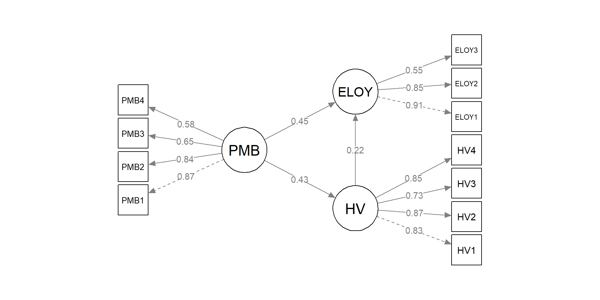
Data E-Loyalty (Khoa & Nguyen, 2020): PMB → HV → ELOY.

dat <- read_excel("data/sem/data.xlsx") |> select(-No)
glimpse(dat)

Rows: 485
Columns: 14
$ HV1        <dbl> 5, 4, 5, 5, 4, 5, 4, 5, 4, 4, 5, 4, 5, 2, 4, 4, 5, 5, 4, 4,…
$ HV2        <dbl> 5, 4, 4, 5, 4, 4, 4, 4, 5, 4, 5, 4, 5, 2, 4, 4, 5, 5, 5, 4,…
$ HV3        <dbl> 5, 4, 5, 4, 4, 5, 4, 4, 4, 3, 5, 4, 5, 2, 4, 4, 5, 5, 4, 4,…
$ HV4        <dbl> 5, 4, 5, 5, 4, 5, 4, 5, 5, 4, 5, 4, 5, 2, 3, 4, 4, 4, 4, 5,…
$ PMB1       <dbl> 4, 4, 4, 4, 5, 4, 3, 4, 4, 4, 4, 4, 4, 3, 4, 4, 4, 5, 5, 4,…
$ PMB2       <dbl> 4, 4, 4, 4, 4, 4, 3, 4, 4, 4, 4, 4, 4, 3, 3, 4, 3, 4, 5, 4,…
$ PMB3       <dbl> 4, 4, 4, 4, 5, 3, 3, 4, 4, 4, 4, 4, 4, 3, 3, 4, 3, 3, 5, 4,…
$ PMB4       <dbl> 4, 4, 4, 4, 4, 4, 3, 4, 3, 3, 4, 4, 4, 3, 3, 3, 4, 3, 4, 4,…
$ ELOY1      <dbl> 5, 4, 4, 4, 4, 5, 3, 3, 5, 4, 4, 3, 3, 3, 4, 3, 5, 5, 3, 4,…
$ ELOY2      <dbl> 5, 4, 4, 4, 4, 4, 3, 3, 4, 4, 4, 3, 3, 3, 3, 3, 5, 5, 3, 4,…
$ ELOY3      <dbl> 4, 5, 4, 4, 4, 4, 4, 4, 5, 5, 4, 4, 5, 3, 3, 4, 4, 5, 4, 5,…
$ gender     <dbl> 2, 2, 1, 2, 2, 1, 2, 2, 1, 2, 1, 1, 1, 1, 1, 2, 2, 1, 1, 1,…
$ occupation <dbl> 4, 6, 3, 5, 1, 5, 5, 2, 1, 4, 7, 4, 6, 5, 2, 3, 6, 3, 5, 5,…
$ times      <dbl> 3, 4, 3, 1, 4, 4, 3, 2, 3, 4, 1, 4, 4, 2, 1, 2, 4, 4, 1, 1,…

Konstruk dan Hipotesis

Konstruk	Indikator	Deskripsi
PMB	PMB1–4	Perceived Mental Benefits
HV	HV1–4	Hedonic Value
ELOY	ELOY1–3	Electronic Loyalty

No	Hipotesis	Path
H1	PMB → ELOY	`ELOY ~ PMB`
H2	PMB → HV	`HV ~ PMB`
H3	HV → ELOY	`ELOY ~ HV`

Sintaks lavaan

Operator	Makna	Contoh
`=~`	“diukur oleh”	`PMB =~ PMB1 + PMB2`
`~`	“diregresikan terhadap”	`ELOY ~ PMB + HV`
`~~`	kovarians/varians	`HV ~~ ELOY`
`:=`	defined parameter	`indirect := a*b`

CFA: Spesifikasi & Estimasi

cfa_model <- '
  PMB  =~ PMB1 + PMB2 + PMB3 + PMB4
  HV   =~ HV1 + HV2 + HV3 + HV4
  ELOY =~ ELOY1 + ELOY2 + ELOY3
'
cfa_fit <- cfa(cfa_model, data = dat)

Fit Indices CFA

fitMeasures(cfa_fit, c("chisq", "df", "pvalue",
                        "cfi", "tli", "rmsea", "srmr"))

  chisq      df  pvalue     cfi     tli   rmsea    srmr 
969.080  41.000   0.000   0.742   0.654   0.216   0.124

Indeks	Kriteria Baik
CFI	≥ 0.90
TLI	≥ 0.90
RMSEA	≤ 0.08
SRMR	≤ 0.08

Tip

Laporkan minimal CFI, RMSEA, dan SRMR. Jangan hanya mengandalkan satu indeks.

Modification Indices

mi <- modindices(cfa_fit, sort = TRUE, minimum.value = 10)
mi |> head(10) |> kable(digits = 3)

	lhs	op	rhs	mi	epc	sepc.lv	sepc.all	sepc.nox
57	PMB1		HV4	134.385	-0.115	-0.115	-0.769	-0.769
45	ELOY	=~	PMB3	133.769	-0.492	-0.390	-0.571	-0.571
43	ELOY	=~	PMB1	109.088	0.433	0.343	0.466	0.466
35	PMB	=~	ELOY3	106.494	0.579	0.370	0.550	0.550
103	ELOY1		ELOY2	93.921	0.507	0.507	3.742	3.742
75	PMB3		ELOY1	91.513	-0.125	-0.125	-0.658	-0.658
66	PMB2		HV4	74.743	0.067	0.067	0.540	0.540
61	PMB2		PMB3	64.859	0.092	0.092	0.588	0.588
31	PMB	=~	HV3	57.716	-0.343	-0.219	-0.307	-0.307
29	PMB	=~	HV1	55.761	0.317	0.203	0.269	0.269

Kolom mi = penurunan chi-square jika parameter ditambahkan. Hanya tambahkan yang punya justifikasi teoretis.

Standardized Loadings

parameterEstimates(cfa_fit, standardized = TRUE) |>
  filter(op == "=~") |>
  select(Konstruk = lhs, Indikator = rhs,
         Loading = est, Std.Loading = std.all, p = pvalue) |>
  mutate(Memadai = ifelse(Std.Loading >= 0.50, "Ya", "Tidak")) |>
  kable(digits = 3)

Konstruk	Indikator	Loading	Std.Loading	p	Memadai
PMB	PMB1	1.000	0.868	NA	Ya
PMB	PMB2	0.733	0.841	0	Ya
PMB	PMB3	0.698	0.652	0	Ya
PMB	PMB4	0.558	0.577	0	Ya
HV	HV1	1.000	0.828	NA	Ya
HV	HV2	0.991	0.873	0	Ya
HV	HV3	0.840	0.734	0	Ya
HV	HV4	1.049	0.847	0	Ya
ELOY	ELOY1	1.000	0.908	NA	Ya
ELOY	ELOY2	0.741	0.847	0	Ya
ELOY	ELOY3	0.464	0.546	0	Ya

Loading ≥ 0.50 memadai, idealnya ≥ 0.70.

CR & AVE

std_loadings <- parameterEstimates(cfa_fit, standardized = TRUE) |>
  filter(op == "=~") |> select(lhs, std.all)

reliabilitas <- std_loadings |>
  group_by(Konstruk = lhs) |>
  summarize(
    n_items = n(),
    AVE = sum(std.all^2) / n(),
    CR = sum(std.all)^2 / (sum(std.all)^2 + (n() - sum(std.all^2))),
    .groups = "drop"
  )
reliabilitas |> kable(digits = 3)

Konstruk	n_items	AVE	CR
ELOY	3	0.613	0.820
HV	4	0.676	0.893
PMB	4	0.555	0.829

AVE ≥ 0.50 (convergent validity), CR ≥ 0.70 (reliabilitas).

Discriminant Validity: Fornell-Larcker

cor_lv <- lavInspect(cfa_fit, "cor.lv")
round(cor_lv, 3)

       PMB    HV  ELOY
PMB  1.000            
HV   0.434 1.000      
ELOY 0.548 0.413 1.000

sqrt_ave <- sqrt(setNames(reliabilitas$AVE, reliabilitas$Konstruk))
round(sqrt_ave, 3)

 ELOY    HV   PMB 
0.783 0.822 0.745

√AVE harus > korelasi antar konstruk pada baris/kolomnya.

Model Tanpa Mediasi

sem_direct <- '
  PMB  =~ PMB1 + PMB2 + PMB3 + PMB4
  HV   =~ HV1 + HV2 + HV3 + HV4
  ELOY =~ ELOY1 + ELOY2 + ELOY3
  ELOY ~ PMB + HV
'
sem_direct_fit <- sem(sem_direct, data = dat)

parameterEstimates(sem_direct_fit, standardized = TRUE) |>
  filter(op == "~") |>
  select(DV = lhs, IV = rhs, B = est, Beta = std.all, p = pvalue) |>
  kable(digits = 3)

DV	IV	B	Beta	p
ELOY	PMB	0.564	0.454	0
ELOY	HV	0.275	0.216	0

Full SEM dengan Mediasi

sem_model <- '
  PMB  =~ PMB1 + PMB2 + PMB3 + PMB4
  HV   =~ HV1 + HV2 + HV3 + HV4
  ELOY =~ ELOY1 + ELOY2 + ELOY3
  HV   ~ a*PMB
  ELOY ~ c*PMB + b*HV
  indirect := a*b
  total    := c + a*b
'

Label a, b, c untuk menghitung indirect & total effect.

Estimasi Bootstrap

sem_fit <- sem(sem_model, data = dat, se = "bootstrap", bootstrap = 1000)

Bootstrap: distribusi sampling mediasi umumnya skewed → CI empiris lebih valid.

Path Coefficients

parameterEstimates(sem_fit, standardized = TRUE) |>
  filter(op == "~") |>
  select(DV = lhs, IV = rhs, B = est, SE = se,
         p = pvalue, Beta = std.all) |>
  mutate(Sig = ifelse(p < 0.05, "Ya", "Tidak")) |>
  kable(digits = 3)

DV	IV	B	SE	Beta	Sig
HV	PMB	0.424	0.081	0.434	Ya
ELOY	PMB	0.564	0.116	0.454	Ya
ELOY	HV	0.275	0.067	0.216	Ya

R² & Mediasi

lavInspect(sem_fit, "r2")

 PMB1  PMB2  PMB3  PMB4   HV1   HV2   HV3   HV4 ELOY1 ELOY2 ELOY3    HV  ELOY 
0.754 0.708 0.426 0.333 0.685 0.763 0.539 0.718 0.824 0.717 0.298 0.188 0.339

parameterEstimates(sem_fit) |>
  filter(op == ":=") |>
  select(Label = label, Estimate = est, p = pvalue,
         CI.Lower = ci.lower, CI.Upper = ci.upper) |>
  kable(digits = 3)

Label	Estimate	p	CI.Lower	CI.Upper
indirect	0.116	0.003	0.054	0.203
total	0.680	0.000	0.491	0.841

CI tidak melewati nol → mediasi signifikan. Efek langsung tetap signifikan → mediasi parsial.

Path Diagram

semPaths(sem_fit, whatLabels = "std", layout = "tree2",
         edge.label.cex = 0.8, style = "lisrel", residuals = FALSE,
         rotation = 2, nCharNodes = 4, sizeMan = 6, sizeLat = 9)

Bagian B: PLS-SEM dengan seminr

library(seminr)

Mengapa PLS-SEM?

Tidak memerlukan asumsi normalitas
Sampel kecil (>50)
Mendukung indikator formatif dan reflektif
Cocok untuk model kompleks
Fokus pada prediksi

Reflektif vs Formatif

Reflektif (Mode A): Indikator = efek dari konstruk. Hapus satu → makna tetap.
Formatif (Mode B): Indikator membentuk konstruk. Hapus satu → makna berubah.

Tipe Konstruk di `seminr`

Fungsi	Model	Penjelasan
`composite()`	Composite Mode A	Default PLS-SEM, correlation weights
`composite(..., mode_B)`	Composite Mode B	Formatif, regression weights
`reflective()`	Common factor	PLSc (consistent PLS)
`higher_composite()`	HOC	Dibentuk dari dimensi konstruk lain
`single_item()`	Single item	Satu indikator

Dataset & Model

mobi <- read_excel("data/plssem/sem_mobi.xlsx")

Konstruk	Indikator	Tipe
Image	IMAG1–3	composite Mode A
Value	PERV1–2	composite Mode A
Satisfaction	HOC	higher_composite (Image + Value)
Quality	PERQ1–3	composite Mode B (formatif)
Complaints	CUSCO	single_item
Loyalty	CUSL1–3	reflective (PLSc)

Hipotesis PLS

No	Hipotesis	Path
H1	Quality → Satisfaction
H2	Satisfaction → Complaints
H3	Satisfaction → Loyalty

Mediasi: Quality → Satisfaction → Loyalty

Spesifikasi Model

mm <- constructs(
  composite("Image",        multi_items("IMAG", 1:3)),
  composite("Value",        multi_items("PERV", 1:2)),
  higher_composite("Satisfaction",
                   dimensions = c("Image", "Value"),
                   method = two_stage),
  composite("Quality",      multi_items("PERQ", 1:3), weights = mode_B),
  composite("Complaints",   single_item("CUSCO")),
  reflective("Loyalty",     multi_items("CUSL", 1:3))
)

sm <- relationships(
  paths(from = "Quality",      to = "Satisfaction"),
  paths(from = "Satisfaction", to = c("Complaints", "Loyalty"))
)

Estimasi PLS

pls_model <- estimate_pls(
  data = as.data.frame(mobi),
  measurement_model = mm,
  structural_model = sm
)

# Workaround bug seminr: HOC dimensions
hoc_dims <- c("Image", "Value")
stage1_scores <- pls_model$first_stage_model$construct_scores
pls_model$rawdata <- cbind(pls_model$rawdata,
                           stage1_scores[, hoc_dims, drop = FALSE])

pls_summary <- summary(pls_model)

Reliabilitas

pls_summary$reliability

             alpha  rhoC   AVE  rhoA
Quality      0.718 0.836 0.633 1.000
Satisfaction 0.640 0.847 0.735 0.641
Complaints   1.000 1.000 1.000 1.000
Loyalty      0.472 0.580 0.368 0.715
Image        0.514 0.754 0.512 0.555
Value        0.824 0.918 0.848 0.861

Alpha, rhoC, and rhoA should exceed 0.7 while AVE should exceed 0.5

rhoC ≥ 0.70, AVE ≥ 0.50. Alpha/rhoA tidak relevan untuk konstruk formatif (Mode B).

Outer Loadings

pls_summary$loadings

      Quality Satisfaction Complaints Loyalty Image Value
Image   0.000        0.866      0.000   0.000 0.000 0.000
Value   0.000        0.848      0.000   0.000 0.000 0.000
PERQ1   0.882        0.000      0.000   0.000 0.000 0.000
PERQ2   0.673        0.000      0.000   0.000 0.000 0.000
PERQ3   0.818        0.000      0.000   0.000 0.000 0.000
CUSCO   0.000        0.000      1.000   0.000 0.000 0.000
CUSL1   0.000        0.000      0.000   0.638 0.000 0.000
CUSL2   0.000        0.000      0.000   0.160 0.000 0.000
CUSL3   0.000        0.000      0.000   0.820 0.000 0.000
IMAG1   0.000        0.000      0.000   0.000 0.832 0.000
IMAG2   0.000        0.000      0.000   0.000 0.720 0.000
IMAG3   0.000        0.000      0.000   0.000 0.569 0.000
PERV1   0.000        0.000      0.000   0.000 0.000 0.900
PERV2   0.000        0.000      0.000   0.000 0.000 0.941

Loading ≥ 0.70 ideal. Loading 0.40–0.70: pertimbangkan dampak pada AVE.

HTMT (Discriminant Validity)

pls_summary$validity$htmt

             Quality Satisfaction Complaints Loyalty Image Value
Quality            .            .          .       .     .     .
Satisfaction   1.011            .          .       .     .     .
Complaints     0.567        0.549          .       .     .     .
Loyalty        0.866        0.947      0.561       .     .     .
Image          1.060        1.491      0.534   0.812     .     .
Value          0.667        1.177      0.387   0.797 0.720     .

HTMT < 0.90 memadai (konservatif: < 0.85). Image–Satisfaction dan Value–Satisfaction tinggi karena mereka dimensi HOC.

Bootstrap

set.seed(2026)
boot <- bootstrap_model(pls_model, nboot = 100, cores = 1)
boot_sum <- summary(boot)

Tip

Minimal nboot = 5000 untuk hasil stabil (Hair et al., 2019). 100 hanya untuk demo.

Path Coefficients (Bootstrap)

boot_sum$bootstrapped_paths

                             Original Est. Bootstrap Mean Bootstrap SD T Stat.
Quality  ->  Satisfaction            0.867          0.878        0.066  13.059
Satisfaction  ->  Complaints         0.549          0.544        0.075   7.306
Satisfaction  ->  Loyalty            0.838          0.853        0.096   8.692
                             2.5% CI 97.5% CI
Quality  ->  Satisfaction      0.760    0.991
Satisfaction  ->  Complaints   0.390    0.662
Satisfaction  ->  Loyalty      0.665    1.072

T > 1.96 dan CI tidak melewati nol → signifikan.

R² dan f²

pls_summary$paths

             Satisfaction Complaints Loyalty
R^2                 0.752      0.302   0.702
AdjR^2              0.751      0.299   0.701
Quality             0.867          .       .
Satisfaction            .      0.549   0.838

R²	Interpretasi
≥ 0.75	Substansial
≥ 0.50	Moderat
≥ 0.25	Lemah

pls_summary$fSquare

             Quality Satisfaction Complaints Loyalty
Quality        0.000        3.035      0.000   0.000
Satisfaction   0.000        0.000      0.432   2.355
Complaints     0.000        0.000      0.000   0.000
Loyalty        0.000        0.000      0.000   0.000

f²: 0.02 kecil, 0.15 sedang, 0.35 besar.

Mediasi PLS-SEM

med1 <- specific_effect_significance(boot,
  from = "Quality", through = "Satisfaction", to = "Loyalty")
med1

 Original Est. Bootstrap Mean   Bootstrap SD        T Stat.        2.5% CI 
     0.7266103      0.7532250      0.1293329      5.6181415      0.5174600 
      97.5% CI 
     1.0304410

med2 <- specific_effect_significance(boot,
  from = "Quality", through = "Satisfaction", to = "Complaints")
med2

 Original Est. Bootstrap Mean   Bootstrap SD        T Stat.        2.5% CI 
    0.47625492     0.47808021     0.07855439     6.06274138     0.32062412 
      97.5% CI 
    0.62451842

PLSpredict

# PLSpredict belum mendukung higher_composite()
# Demo dengan model sederhana tanpa HOC:
mm_simple <- constructs(
  composite("Quality",      multi_items("PERQ", 1:3), weights = mode_B),
  composite("Satisfaction", multi_items("IMAG", 1:3)),
  composite("Complaints",   single_item("CUSCO")),
  reflective("Loyalty",     multi_items("CUSL", 1:3))
)
sm_simple <- relationships(
  paths(from = "Quality",      to = "Satisfaction"),
  paths(from = "Satisfaction", to = c("Complaints", "Loyalty"))
)
pls_simple <- estimate_pls(data = as.data.frame(mobi),
                           measurement_model = mm_simple,
                           structural_model = sm_simple)
set.seed(2026)
pred <- predict_pls(pls_simple, technique = predict_DA, noFolds = 10)
summary(pred)


PLS in-sample metrics:
     IMAG1 IMAG2 IMAG3 CUSCO CUSL1 CUSL2 CUSL3
RMSE 1.489 1.414 2.058 2.105 2.525 2.829 2.006
MAE  1.081 1.047 1.547 1.595 1.910 2.387 1.474

PLS out-of-sample metrics:
     IMAG1 IMAG2 IMAG3 CUSCO CUSL1 CUSL2 CUSL3
RMSE 1.504 1.446 2.075 2.137 2.564 2.848 2.034
MAE  1.090 1.065 1.561 1.621 1.940 2.401 1.487

LM in-sample metrics:
     IMAG1 IMAG2 IMAG3 CUSCO CUSL1 CUSL2 CUSL3
RMSE 1.432 1.327 1.980 2.039 2.494 2.816 1.973
MAE  1.044 0.997 1.482 1.579 1.915 2.378 1.481

LM out-of-sample metrics:
     IMAG1 IMAG2 IMAG3 CUSCO CUSL1 CUSL2 CUSL3
RMSE 1.458 1.367 2.022 2.090 2.548 2.874 2.014
MAE  1.059 1.025 1.511 1.624 1.955 2.430 1.502

Construct Level metrics:
        Satisfaction Complaints Loyalty
IS_MSE        0.6161     0.8578   0.854
IS_MAE        0.5785     0.7019   0.656
OOS_MSE       0.6373     0.8721   0.878
OOS_MAE       0.5854     0.7073   0.665
overfit       0.0343     0.0167   0.028

PLS RMSE < LM RMSE → predictive power baik.

Path Diagram PLS

plot(boot)

save_plot("plsem.png")

Rekap Sesi 3

Perbandingan Praktis

Aspek	CB-SEM (`lavaan`)	PLS-SEM (`seminr`)
Sintaks	`=~`, `~`	`constructs()`, `relationships()`
Estimasi	`cfa()` / `sem()`	`estimate_pls()`
Signifikansi	Langsung dari output	`bootstrap_model()`
Fit indices	CFI, TLI, RMSEA, SRMR	R², f², HTMT
Mediasi	Label + `:=`	`specific_effect_significance()`

Yang Sudah Dipelajari

Konsep SEM: laten vs manifes, measurement vs structural
CB-SEM: CFA → Full SEM, fit indices, CR, AVE, Fornell-Larcker, mediasi
PLS-SEM: composite (Mode A/B), reflective (PLSc), HOC, single_item, bootstrap, R², f², HTMT

Latihan

Latihan 1: CB-SEM

Hapus path ELOY ~ HV dan estimasi ulang.

Jawaban

sem_model2 <- '
  PMB  =~ PMB1 + PMB2 + PMB3 + PMB4
  HV   =~ HV1 + HV2 + HV3 + HV4
  ELOY =~ ELOY1 + ELOY2 + ELOY3
  HV   ~ PMB
  ELOY ~ PMB
'
sem_fit2 <- sem(sem_model2, data = dat)
fitMeasures(sem_fit2, c("cfi", "tli", "rmsea", "srmr"))

  cfi   tli rmsea  srmr 
0.742 0.654 0.216 0.124

Latihan 2: PLS-SEM

Hapus CUSL2 dari Loyalty, estimasi ulang. Apakah reliabilitas membaik?

Jawaban

mm2 <- constructs(
  composite("Image",        multi_items("IMAG", 1:3)),
  composite("Value",        multi_items("PERV", 1:2)),
  higher_composite("Satisfaction",
                   dimensions = c("Image", "Value"),
                   method = two_stage),
  composite("Quality",      multi_items("PERQ", 1:3), weights = mode_B),
  composite("Complaints",   single_item("CUSCO")),
  reflective("Loyalty",     c("CUSL1", "CUSL3"))
)
pls_model2 <- estimate_pls(
  data = as.data.frame(mobi),
  measurement_model = mm2,
  structural_model = sm
)
stage1 <- pls_model2$first_stage_model$construct_scores
for (d in c("Image", "Value")) {
  pls_model2$rawdata[[d]] <- stage1[, d]
}
summary(pls_model2)$reliability

             alpha  rhoC   AVE  rhoA
Quality      0.718 0.837 0.633 1.000
Satisfaction 0.640 0.847 0.735 0.641
Complaints   1.000 1.000 1.000 1.000
Loyalty      0.703 0.714 0.559 0.733
Image        0.514 0.754 0.512 0.556
Value        0.824 0.918 0.848 0.866

Alpha, rhoC, and rhoA should exceed 0.7 while AVE should exceed 0.5

Akhir Sesi 3!

Terima kasih atas partisipasinya!

Structural Equation Modelling (SEM)

Rencana Hari Ini

Apa itu SEM?

Terminologi SEM

CB-SEM vs PLS-SEM

Two-Step Approach

Bagian A: CB-SEM dengan lavaan

Import Data

Konstruk dan Hipotesis

Sintaks lavaan

CFA: Spesifikasi & Estimasi

Fit Indices CFA

Modification Indices

Standardized Loadings

CR & AVE

Discriminant Validity: Fornell-Larcker

Model Tanpa Mediasi

Full SEM dengan Mediasi

Estimasi Bootstrap

Path Coefficients

R² & Mediasi

Path Diagram

Bagian B: PLS-SEM dengan seminr

Mengapa PLS-SEM?

Reflektif vs Formatif

Tipe Konstruk di seminr

Dataset & Model

Hipotesis PLS

Spesifikasi Model

Estimasi PLS

Reliabilitas

Outer Loadings

HTMT (Discriminant Validity)

Bootstrap

Path Coefficients (Bootstrap)

R² dan f²

Mediasi PLS-SEM

PLSpredict

Path Diagram PLS

Rekap Sesi 3

Perbandingan Praktis

Yang Sudah Dipelajari

Latihan

Latihan 1: CB-SEM

Latihan 2: PLS-SEM

Akhir Sesi 3!

Tipe Konstruk di `seminr`