[1] 6922Analisis Regresi
ISEI Workshop
Rencana Hari Ini
Bagian 1: Regresi Linear Sederhana
- Konsep regresi dan korelasi
- Model regresi sederhana, interpretasi koefisien
Bagian 2: Regresi Linear Berganda
- Menambahkan prediktor, ANOVA, diagnostik
Bagian 3: Variabel Kategorikal dan Pelaporan
- Dummy variable, interaksi, pelaporan
Apa itu Regresi?
\[Y = \beta_0 + \beta_1 X_1 + \beta_2 X_2 + \ldots + \beta_p X_p + \varepsilon\]
| Komponen | Simbol | Makna |
|---|---|---|
| Intercept | \(\beta_0\) | Nilai Y ketika semua X = 0 |
| Slope | \(\beta_k\) | Perubahan Y per kenaikan 1 unit \(X_k\) |
| Error | \(\varepsilon\) | Selisih prediksi dan aktual |
Tujuan OLS: Menemukan garis terbaik yang meminimalkan jumlah kuadrat error.
Korelasi vs Regresi
- Korelasi: kekuatan dan arah hubungan (simetris: \(r_{xy} = r_{yx}\))
- Regresi: memprediksi Y berdasarkan X (tidak simetris)
- Korelasi bukan kausalitas!
Di R: lm(Y ~ X1 + X2) — simbol ~ = “diprediksi oleh”, + = menambah prediktor.
Asumsi Regresi Linear
- Linearitas: hubungan X dan Y linear
- Independensi: residual saling independen
- Homoskedastisitas: varians residual konstan
- Normalitas: residual berdistribusi normal
- Multikolinearitas: prediktor tidak terlalu berkorelasi
Landasan Teori
- SWB (Diener et al., 1999): evaluasi kognitif dan afektif terhadap kehidupan
- Kebebasan (Inglehart, 2000; Sen, 1999): prediktor penting kesejahteraan subjektif
- Skala ordinal sebagai kontinu (Norman, 2010): skala Likert ≥ 5 poin dapat diperlakukan sebagai data kontinu
Import & Pembersihan Data
Bagian 1: Regresi Linear Sederhana
Korelasi
[1] 0.6472145
Pearson's product-moment correlation
data: dat$kepuasan_finansial and dat$kepuasan_hidup
t = 70.627, df = 6920, p-value < 2.2e-16
alternative hypothesis: true correlation is not equal to 0
95 percent confidence interval:
0.6333125 0.6606990
sample estimates:
cor
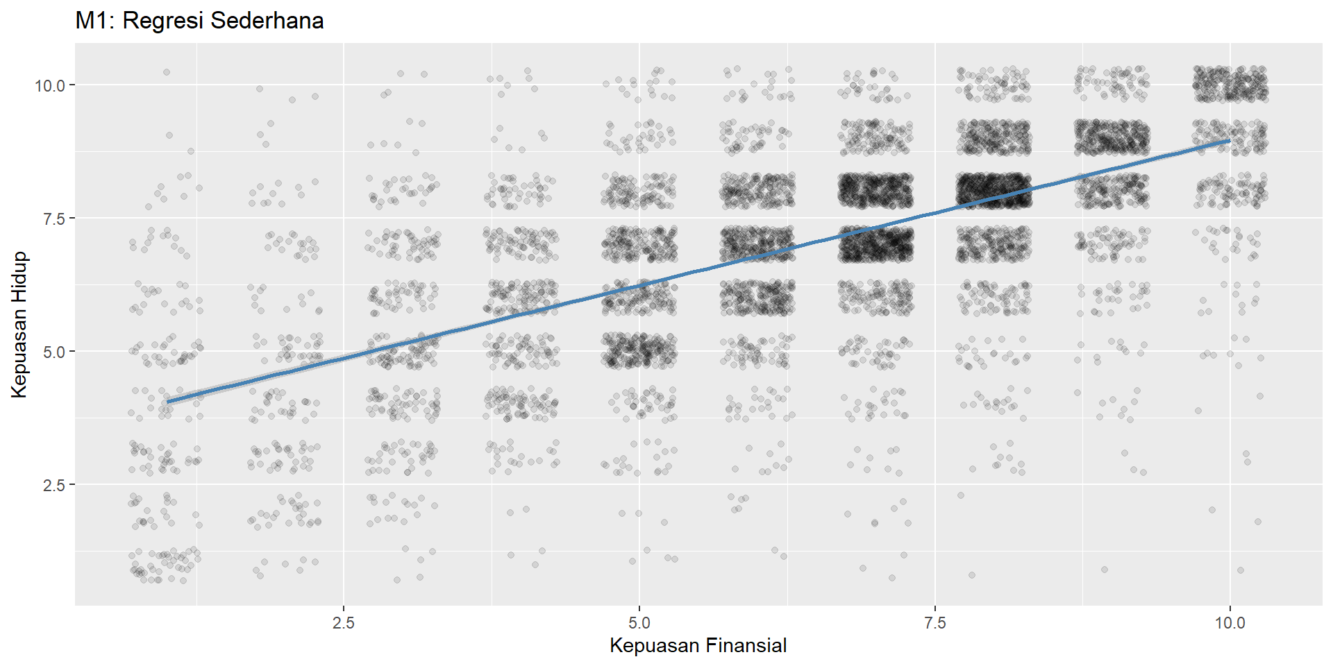
0.6472145 Model Sederhana (M1)
# A tibble: 2 × 7
  term               estimate std.error statistic p.value conf.low conf.high
  <chr>                 <dbl>     <dbl>     <dbl>   <dbl>    <dbl>     <dbl>
1 (Intercept)           3.51    0.0535       65.7       0    3.41      3.62
2 kepuasan_finansial 0.545 0.00772 70.6 0 0.530 0.560- Intercept = 3.51: prediksi jika kepuasan finansial = 0
- Slope = 0.545: setiap +1 poin finansial → +0.545 poin kepuasan hidup
R-squared
# A tibble: 1 × 3
  r.squared adj.r.squared    AIC
      <dbl>         <dbl>  <dbl>
1     0.419         0.419 24222.
\(R^2\) = proporsi varians Y yang dijelaskan model (0–1). \(R^2_{adj}\) disesuaikan jumlah prediktor.
Visualisasi M1
Visualisasi M1
Bagian 2: Regresi Linear Berganda
Model 2 Prediktor (M2)
# A tibble: 3 × 7
  term               estimate std.error statistic   p.value conf.low conf.high
  <chr>                 <dbl>     <dbl>     <dbl>     <dbl>    <dbl>     <dbl>
1 (Intercept)           1.71    0.0648       26.3 8.78e-146    1.58      1.83
2 kepuasan_finansial    0.388   0.00788      49.2 0            0.373     0.404
3 kebebasan_memilih     0.388   0.00940      41.3 0            0.370     0.407
Important
Setiap koefisien diinterpretasikan “dengan mengontrol variabel lain” (ceteris paribus).
Model Penuh (M3)
# A tibble: 5 × 7
  term               estimate std.error statistic  p.value conf.low conf.high
  <chr>                 <dbl>     <dbl>     <dbl>    <dbl>    <dbl>     <dbl>
1 (Intercept)         1.31     0.0781       16.8  3.07e-62  1.16      1.47
2 kepuasan_finansial  0.379    0.00792      47.9  0         0.364     0.395
3 kebebasan_memilih   0.389    0.00935      41.6  0         0.371     0.407
4 religiusitas        0.0323   0.00578       5.59 2.39e- 8  0.0210    0.0436
5 usia                0.00569  0.000894      6.37 2.02e-10  0.00394   0.00744
Bagian 3: Variabel Kategorikal dan Interaksi
Dummy Variables (M4)
R otomatis membuat dummy dari factor. Kategori referensi: level pertama.
| term | estimate | std.error | statistic | p.value | conf.low | conf.high |
|---|---|---|---|---|---|---|
| (Intercept) | 1.293 | 0.080 | 16.217 | 0.000 | 1.136 | 1.449 |
| kepuasan_finansial | 0.379 | 0.008 | 47.885 | 0.000 | 0.364 | 0.395 |
| kebebasan_memilih | 0.389 | 0.009 | 41.567 | 0.000 | 0.370 | 0.407 |
| religiusitas | 0.032 | 0.006 | 5.505 | 0.000 | 0.021 | 0.043 |
| usia | 0.006 | 0.001 | 6.451 | 0.000 | 0.004 | 0.008 |
| jenis_kelaminPerempuan | 0.040 | 0.030 | 1.348 | 0.178 | -0.018 | 0.099 |
Model dengan Negara (M5)
| term | estimate | std.error | statistic | p.value | conf.low | conf.high |
|---|---|---|---|---|---|---|
| (Intercept) | 1.256 | 0.081 | 15.541 | 0.000 | 1.098 | 1.414 |
| kepuasan_finansial | 0.377 | 0.008 | 47.548 | 0.000 | 0.361 | 0.392 |
| kebebasan_memilih | 0.394 | 0.009 | 41.623 | 0.000 | 0.376 | 0.413 |
| religiusitas | 0.028 | 0.006 | 4.679 | 0.000 | 0.016 | 0.039 |
| usia | 0.005 | 0.001 | 5.781 | 0.000 | 0.003 | 0.007 |
| jenis_kelaminPerempuan | 0.031 | 0.030 | 1.028 | 0.304 | -0.028 | 0.090 |
| negaraSelandia Baru | 0.151 | 0.046 | 3.275 | 0.001 | 0.060 | 0.241 |
| negaraSingapura | 0.156 | 0.035 | 4.427 | 0.000 | 0.087 | 0.225 |
Mengubah Kategori Referensi
| term | estimate | std.error | statistic | p.value | conf.low | conf.high |
|---|---|---|---|---|---|---|
| (Intercept) | 1.412 | 0.083 | 16.969 | 0.000 | 1.249 | 1.575 |
| kepuasan_finansial | 0.377 | 0.008 | 47.548 | 0.000 | 0.361 | 0.392 |
| kebebasan_memilih | 0.394 | 0.009 | 41.623 | 0.000 | 0.376 | 0.413 |
| religiusitas | 0.028 | 0.006 | 4.679 | 0.000 | 0.016 | 0.039 |
| usia | 0.005 | 0.001 | 5.781 | 0.000 | 0.003 | 0.007 |
| jenis_kelaminPerempuan | 0.031 | 0.030 | 1.028 | 0.304 | -0.028 | 0.090 |
| negaraKanada | -0.156 | 0.035 | -4.427 | 0.000 | -0.225 | -0.087 |
| negaraSelandia Baru | -0.005 | 0.051 | -0.104 | 0.917 | -0.105 | 0.094 |
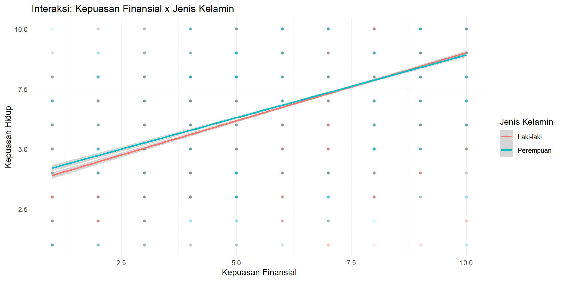
Model Interaksi (M6)
Interaksi: efek satu variabel tergantung level variabel lain.
| term | estimate | std.error | statistic | p.value | conf.low | conf.high |
|---|---|---|---|---|---|---|
| (Intercept) | 1.198 | 0.092 | 13.075 | 0.000 | 1.018 | 1.377 |
| kepuasan_finansial | 0.394 | 0.011 | 37.055 | 0.000 | 0.373 | 0.415 |
| jenis_kelaminPerempuan | 0.231 | 0.095 | 2.418 | 0.016 | 0.044 | 0.418 |
| kebebasan_memilih | 0.388 | 0.009 | 41.504 | 0.000 | 0.370 | 0.407 |
| religiusitas | 0.032 | 0.006 | 5.488 | 0.000 | 0.020 | 0.043 |
| usia | 0.006 | 0.001 | 6.469 | 0.000 | 0.004 | 0.008 |
| kepuasan_finansial:jenis_kelaminPerempuan | -0.029 | 0.014 | -2.101 | 0.036 | -0.056 | -0.002 |
Visualisasi Interaksi
Visualisasi Interaksi
Bagian 4: Diagnostik dan Perbandingan Model
ANOVA: Perbandingan Model
Analysis of Variance Table

Model 1: kepuasan_hidup ~ kepuasan_finansial
Model 2: kepuasan_hidup ~ kepuasan_finansial + kebebasan_memilih
Model 3: kepuasan_hidup ~ kepuasan_finansial + kebebasan_memilih + religiusitas +
    usia
  Res.Df   RSS Df Sum of Sq        F    Pr(>F)
1   6920 13399
2   6919 10750  1   2648.89 1724.066 < 2.2e-16 ***
3   6917 10627  2    122.78   39.956 < 2.2e-16 ***
---
Signif. codes:  0 '***' 0.001 '**' 0.01 '*' 0.05 '.' 0.1 ' ' 1
Model nested: jika p < 0.05, model lebih kompleks signifikan lebih baik.
Tabel Perbandingan (Cohen’s f²)
r2_adj <- c(glance(m1)$adj.r.squared, glance(m2)$adj.r.squared,
            glance(m3)$adj.r.squared, glance(m4)$adj.r.squared,
            glance(m5)$adj.r.squared, glance(m6)$adj.r.squared)

cohens_f2 <- c(NA, diff(r2_adj) / (1 - r2_adj[-1]))

tibble(
  Model = paste0("m", 1:6),
  Formula = c("finansial", "+ kebebasan", "+ religiusitas + usia",
              "+ jenis_kelamin", "+ negara", "finansial * jk + lainnya"),
  R2_adj = r2_adj,
  AIC = c(AIC(m1), AIC(m2), AIC(m3), AIC(m4), AIC(m5), AIC(m6)),
  Cohens_f2 = cohens_f2
) |> kable(digits = 3)| Model | Formula | R2_adj | AIC | Cohens_f2 |
|---|---|---|---|---|
| m1 | finansial | 0.419 | 24221.64 | NA |
| m2 | + kebebasan | 0.534 | 22698.99 | 0.246 |
| m3 | + religiusitas + usia | 0.539 | 22623.47 | 0.011 |
| m4 | + jenis_kelamin | 0.539 | 22623.65 | 0.000 |
| m5 | + negara | 0.540 | 22602.88 | 0.003 |
| m6 | finansial * jk + lainnya | 0.539 | 22621.24 | -0.003 |
Cohen’s f²: 0.02 = kecil, 0.15 = sedang, 0.35 = besar.
Diagnostic Plots
Diagnostic Plots
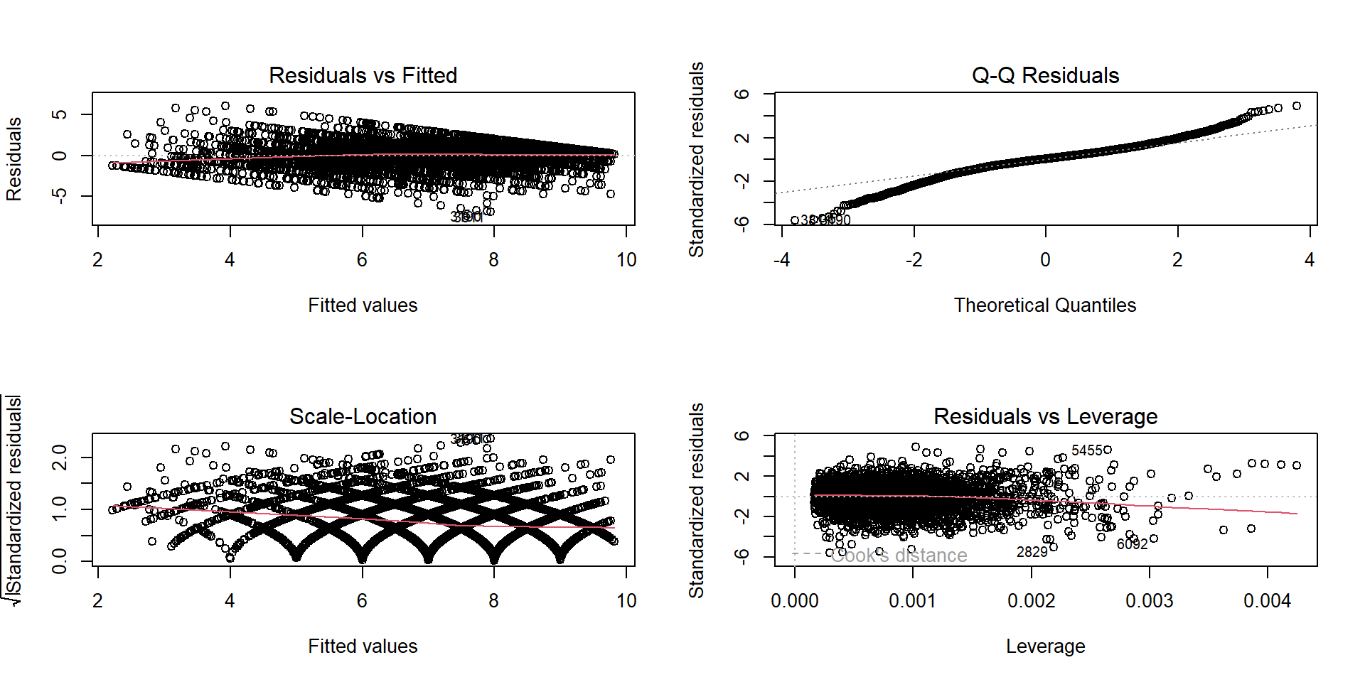
Membaca Diagnostic Plots
- Residuals vs Fitted: linearitas & homoskedastisitas (menyebar acak = baik)
- Normal Q-Q: normalitas residual (ikut garis diagonal = baik)
- Scale-Location: homoskedastisitas (garis datar = baik)
- Residuals vs Leverage: observasi berpengaruh (di luar Cook’s distance = hati-hati)
VIF & Uji Formal
VIF < 5: OK. VIF 5–10: perlu perhatian. VIF > 10: masalah serius.
Uji Normalitas & Autokorelasi
    Asymptotic one-sample Kolmogorov-Smirnov test

data:  m3$residuals
D = 0.066964, p-value < 2.2e-16
alternative hypothesis: two-sided
    Durbin-Watson test

data:  m3
DW = 1.9745, p-value = 0.1432
alternative hypothesis: true autocorrelation is greater than 0
Note
Durbin-Watson dirancang untuk time series. Pada cross-section, autokorelasi bisa muncul jika data diurutkan atau ada clustering.
Uji Heteroskedastisitas
Jika p < 0.05 → heteroskedastisitas terdeteksi.
Robust Standard Errors
t test of coefficients:

                     Estimate Std. Error t value  Pr(>|t|)
(Intercept)        1.31388387 0.08886323 14.7855 < 2.2e-16 ***
kepuasan_finansial 0.37921502 0.01134592 33.4230 < 2.2e-16 ***
kebebasan_memilih  0.38907553 0.01354804 28.7182 < 2.2e-16 ***
religiusitas       0.03228555 0.00580773  5.5591 2.813e-08 ***
usia               0.00569275 0.00093759  6.0717 1.333e-09 ***
---
Signif. codes:  0 '***' 0.001 '**' 0.01 '*' 0.05 '.' 0.1 ' ' 1
Robust SE mengubah inferensi, tidak mengubah koefisien.
Aturan Praktis Robust SE
| Situasi | Rekomendasi |
|---|---|
| Cross-section, n > 250 | HC1 atau HC3 |
| Cross-section, n < 100 | HC3 |
| Panel data (clustered) | Cluster-robust SE |
| Time series + autocorrelation | HAC / Newey-West |
| Ragu? | HC3 — aman untuk mayoritas kasus |
Standardized Coefficients
| term | estimate | std.error | statistic | p.value | conf.low | conf.high |
|---|---|---|---|---|---|---|
| (Intercept) | 0.000 | 0.008 | 0.000 | 1 | -0.016 | 0.016 |
| kepuasan_finansial | 0.450 | 0.009 | 47.870 | 0 | 0.432 | 0.469 |
| kebebasan_memilih | 0.387 | 0.009 | 41.607 | 0 | 0.369 | 0.406 |
| religiusitas | 0.046 | 0.008 | 5.588 | 0 | 0.030 | 0.062 |
| usia | 0.053 | 0.008 | 6.369 | 0 | 0.037 | 0.069 |
\(\beta\) terstandarisasi: prediktor dengan |\(\beta\)| terbesar = pengaruh relatif terkuat.
Pelaporan Hasil
Tips Pelaporan
- Laporkan \(R^2\) adjusted
- Gunakan B (unstandardized) ATAU β (standardized) — konsisten
- Sertakan 95% CI
- Laporkan F-test keseluruhan model
- Sebutkan jumlah observasi
- Variabel tidak signifikan tetap dilaporkan
Rekap Sesi 2
Ringkasan
| Topik | Detail |
|---|---|
| Regresi sederhana | lm(Y ~ X) |
| Regresi berganda | lm(Y ~ X1 + X2 + ...) |
| Interpretasi | B, \(R^2\), p-value, CI |
| Diagnostik | residual plots, VIF, BP test, robust SE |
| Kategorikal | factor(), relevel(), dummy |
| Interaksi | X1 * X2 |
| Perbandingan | ANOVA, AIC, Cohen’s f² |
| Paket | Fungsi Utama |
|---|---|
broom |
tidy(), glance() |
car |
vif() |
lmtest |
bptest(), dwtest(), coeftest() |
sandwich |
vcovHC() |
Latihan
Latihan 1
Model regresi sederhana:
kepuasan_hidup ~ kebebasan_memilih
Jawaban
# A tibble: 2 × 7
  term              estimate std.error statistic   p.value conf.low conf.high
  <chr>                <dbl>     <dbl>     <dbl>     <dbl>    <dbl>     <dbl>
1 (Intercept)          2.64    0.0721       36.6 4.99e-268    2.50      2.78
2 kebebasan_memilih 0.611 0.00958 63.8 0 0.592 0.630# A tibble: 1 × 2
r.squared adj.r.squared
<dbl> <dbl>
1 0.370 0.370Latihan 2
Model regresi berganda penuh + periksa VIF
Jawaban
# A tibble: 5 × 7
  term               estimate std.error statistic  p.value conf.low conf.high
  <chr>                 <dbl>     <dbl>     <dbl>    <dbl>    <dbl>     <dbl>
1 (Intercept)         1.31     0.0781       16.8  3.07e-62  1.16      1.47
2 kepuasan_finansial  0.379    0.00792      47.9  0         0.364     0.395
3 kebebasan_memilih   0.389    0.00935      41.6  0         0.371     0.407
4 religiusitas        0.0323   0.00578       5.59 2.39e- 8  0.0210    0.0436
5 usia 0.00569 0.000894 6.37 2.02e-10 0.00394 0.00744kepuasan_finansial kebebasan_memilih religiusitas usia
1.328704 1.301577 1.012549 1.036567 Latihan 3
Gabungkan
wvs1.xlsxdanwvs2.xlsx, buat model terbaik
Jawaban
wvs2 <- read_excel("data/regresi/wvs2.xlsx")
wvs_all <- bind_rows(wvs, wvs2) |>
  select(kepuasan_hidup, kepuasan_finansial, religiusitas,
         kebebasan_memilih, usia, jenis_kelamin, negara) |>
  drop_na()

m_final <- lm(kepuasan_hidup ~ kepuasan_finansial + kebebasan_memilih +
                religiusitas + usia + jenis_kelamin + negara, data = wvs_all)
tidy(m_final, conf.int = TRUE)
# A tibble: 11 × 7
term estimate std.error statistic p.value conf.low conf.high
<chr> <dbl> <dbl> <dbl> <dbl> <dbl> <dbl>
1 (Intercept) 2.25 0.0791 28.4 1.72e-172 2.09 2.40
2 kepuasan_finansial 0.420 0.00620 67.7 0 0.407 0.432
3 kebebasan_memilih 0.285 0.00685 41.6 0 0.271 0.298
4 religiusitas 0.0207 0.00571 3.63 2.87e- 4 0.00951 0.0319
5 usia 0.00517 0.000863 5.99 2.16e- 9 0.00348 0.00686
6 jenis_kelaminOthers -0.671 0.516 -1.30 1.93e- 1 -1.68 0.339
7 jenis_kelaminPerem… 0.0901 0.0267 3.38 7.30e- 4 0.0378 0.142
8 negaraKanada -0.447 0.0403 -11.1 1.68e- 28 -0.526 -0.368
9 negaraSelandia Baru -0.290 0.0613 -4.74 2.15e- 6 -0.410 -0.170
10 negaraSingapura -0.348 0.0389 -8.94 4.44e- 19 -0.424 -0.271
11 negaraThailand -0.352 0.0523 -6.74 1.62e- 11 -0.455 -0.250 # A tibble: 1 × 3
r.squared adj.r.squared AIC
<dbl> <dbl> <dbl>
1 0.434 0.434 50227.Akhir Sesi 2!
Terima kasih! Sesi berikutnya: Structural Equation Modelling (SEM).